Mohammed Zaheer Ahmed* | Chitraivel Mahesh
© 2021 IIETA. This article is published by IIETA and is licensed under the CC BY 4.0 license (http://creativecommons.org/licenses/by/4.0/).
OPEN ACCESS
The multi-modal health information representing the learning material was examined and multiple learning models were suggested for disease risk assessments, with the aim of mining information from the medical data and developing intelligent applications issues. A medical textual learning model based on a convolution neural network is proposed for the aspect of medical textual functional education. In the framework for risk evaluation, the convolution neural network information retrieval methodology is applied. The deep learning approach is used for medical data representation. To achieve flexibility of the model, the learning and extraction of various disease qualities use the same process. A simple pre-processing of the experimental data samples, including their denigration of power frequency and regulating lead convolution, builds a convolution neural network for advancing and intelligent recognition of medical data. The impressive performance gain achieved by Deep Neural Networks (DNNs) for various tasks prompted us to use DNN for the task of image classification. For the extraction and classification of functions, we used a DNN version called Deep Convolution Neural Network (DCNN). For classification and feature extraction, neural networks can be used. Two related roles can be seen better in our work. DCNN is used for the extraction and classification of functions in the first task. The second task is to extract functions using DCNN, and then to identify extracted characteristics with the SVM classifier. Function extraction shows small features extracted, but image information is useful. One of the major problems for the Content based Image Retrieval (CBIR) is that useful information must be extracted from the raw data to display image contents. The removal task changes the rich content of the image into various functions. The architecture with three levels of concentration and pooling, followed by a complete connected output layer, is used for extraction of functionalities among various configurations that we have considered. DCNN extracted features are supplied in task 1 for classification to a 2 hidden layer neural network. The proposed model is compared with the traditional models and the results show that the performance of the proposed model is better in terms of accuracy levels.
feature extraction, feature selection, medical data clustering, deep neural networks, deep convolution neural network, content based image retrieval
Medical health data is a complex multi-modal data, which keeps increasing fast. It includes a wealth of information. Medical health data issues include how medical health data can be collected and obtained easily and reliably, and how high speed networks are effectively used to carry out medical data. Reliable and efficient communication, how computer education and deep learning techniques relating to artificial intelligence are applied to obtain helpful information from health based big data, and how smart technologies for the majority of medical personnel and ordinary persons are created. Convolution neural systems are an important deeper learning structure and are primarily used for the recognition of two-dimensional images. There are many benefits to the overall neural network itself. For instance, its weight sharing is highly acclaimed.
The subdivision of the neural networks makes the organisation of the neural networks comparable to that of the visual nervous system, which simplifies the neural network by grouping its constituents into smaller clusters. As indicated by the weight on this scale, there has been a significant decrease in weight lifting. Furthermore, because of the inclusion of reconstruction as an ingredient in the equation, the secondary structure of the convolution neural structure makes input as well as the original picture subject to translation, scaling, and rotation. Medical and other types of data, such as embedded sensors, health monitoring systems, cellular sensors, and ambient sensors, comprise large amounts of health care data. The proposed paradigm focuses on multidimensional evaluation both at home and abroad, using a few and diverse elements. Multi-base examination in association with text and medical pictures and results revealed the process advancement in regards to 12 diseases. To finally achieve the representation form for the initial database functions, functional algorithms are used to make the data analyse itself. There is a controlled procedure that is used to learn and gather sample data, and that data transmits from the input to the intended final result layer of the pattern.
Deep knowledge became popular as neural networking began to overdo many high profile pictorial analysis benchmarks. More famously, in 2018, when a deep education model halved the second best image classification error rate, the ImageNet Large-Scale visual recognition challenge (ILSVRC) is considered for image handling and content retrieval. Computers were considered recently to be a very difficult task in the field of natural image recognition but now convolution neural networks have also outnumbered ILSVRC's success by reaching a stage that basically resolves ILSVRC classification tasks with error rate close to the Bayes rate. Deep learning technology has become a norm for a large number of issues with computer vision. They are, however, not restricted to the use of images or analytical methods. They outperform other techniques, such as natural language processing, speech recognition, and analysis of non-structured, tabular data using entity embedding.
Healthcare providers create and collect vast quantities of data containing extremely useful signalling and knowledge, well beyond what "traditional" analytical approaches can manage. This means that machine learning enters into view easily, since it is one of the best ways of integrating, analysing and predicting massive heterogeneous data sets. Deep learning health applications range from the one-dimensional bio signal study, to prediction of clinical decisions and survival studies, to the use of drugs and cardiac arrests, the use of computer aided diagnostics to enhance operational selection, and pharmacogenomics. The method of representing high dimensional data in a lower dimensional space represents a decrease in dimension. It can be interpreted in this step as the projection of data from higher space into lower space. These strategies for reduction of dimensionality are essentially graded according to the projection of data into linear and nonlinear methods.
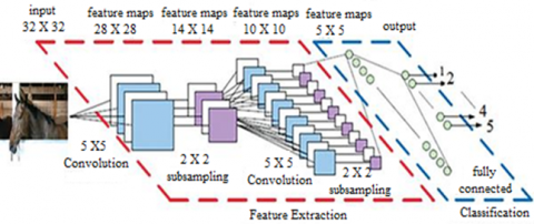
CNN is a type of artificial neural network typically intended to extract data characteristics to classify high dimensional data. A Convolution Neural Network (CNN) is specifically designed for the reorganisation, translation, scaling, skewing and other distortion types in two dimensional form. The structure involves extraction of functions, mapping of functions and subsampling layers. A CNN contains multiple combining and subsampling layers with completely connected output layers optionally. The CNN is biologically inspired versions of the Neural Multilayer Network. The small sub-regions of the visual field, called receptive fields, are susceptible to each cell. There are two types of cells: single cells and complex cells, in which simple cells isolate features and complex cells from a spatial neighbourhood that incorporate some of the local characteristics. In contrast to traditional techniques where features are taken manually and supplied to the models for gradation, CNN attempts to mimic this structure, by extracting features from the input area in a similar manner and then conducting the classification. The CNN framework for feature extraction and classification is represented in Figure 1.
Essentially, the idea is that one community or sub-level category can be divided into subsets or categories while doing a cluster analysis. True cluster structures are unquantified, meaning there is an undefined amount of them, rendering them a total mess in the learning process. clusters to be used in the simulation to allow for more accurate predictions about future galaxies (k). The variables of greatest importance are the ones we cannot identify, and all the other combinations may be left out of consideration. finding the features, and learning how the number of clusters according to the features can be classified.
This paper looks at how to increase the availability of health data to include video, voice, images, and more, and improves the knowledge required for problem solving about diseases by doing so as to broaden the variety of data-oriented medical issues that may be found inside. In the framework for risk evaluation, the convolution neural network text analysis methodology is applied. The deep learning approach is used for medical data representation. To achieve flexibility of the model, the learning and extraction of various disease qualities use the same process. A simple pre-processing of the test data samples, including its regularisation of the power frequency leads, creates a convolution neural network for advancing the medical feature and smart recognition. This was the basis for several experiments to discuss the influence on the experimental results of the convolution kernel and to select learning rates. Comparative testing is also conducted on the support vector machine, neural BP network and neural RBF network.
Figure 1. CNN architecture for feature extraction and classification
Attribute sub setting, attribute collection, or sub setting attributes, function sub setting may be used to either manage the features or to use only the ones that expand the use of the features is important. Since the extracted features would still serve as features, it is an opportunity to increase the inaccuracy, this whole extraction will need more time. Generally, domain awareness is needed for feature extraction. At certain cases, general strategies can help, but at other occasions, it is not possible to provide an exact prediction. Once the features are retrieved, they must be retained to use throughout the selection process. Many different search methods are possible that could be more explored if you know anything about what kinds of features are picked.
More recently, the function search space is being searched by means of genetic algorithms or other biologically-inspired algorithms. with the help of various special-purpose tools, this data processing is accomplished. Approaches to handle a variety of feature selection algorithms and strategies are available for supervised learning. Even, the methods for applying unsupervised attribute extraction to learn are still in their early stages. Now that we are optimizing at our maximum level of potential, we are seeing the most precise outcomes. Once the clusters have been expanded, the data is checked for validity, it is double checked for consistency.
Dimensionality introduces the biggest obstacle to the decision on the path to function expansion. whereas feature selection strategies are called "dimensional reduction" domain. The two methods of calculating factorials are: Transformation-based factorial and Selection-based factorial.
Algorithms were developed and reliable results were obtained from a small subset of medical datasets. For every medical field, the achievement of accurate results was still very difficult for a much larger generalised data set. Kisekka et al. [1] proposed a system expert programme which uses a Bayesian classification to estimate the post-diagnosis probabilities assumed with the symptoms.
Hierarchial clustering is known as the dendrogram for building a cluster hierarchy. Each cluster node consists of clusters for children, siblings divide their common parent's points. The hybrid hierarchical clustering method for the analysis of microarray data has been proposed by Zhao et al. [2]. The research work incorporates both top-down and bottom-up definition of hierarchical clustering in order to use the strengths of this clustering approach [3]. In its study of microarray data, Yin et al. [4] suggested an integrated approach. It uses the hierarchical clustering method to divide patients into two cluster groups, with the expression profile of 192 genes, according to their duration of hospital stay, which increases the hospital's resource management capacity.
Many types of machine learning models are loosely defined by how models use their data during training. In enhancement learning, you create agents who can research and error while optimization of an objective function from their environments. AlphaGo and AlphaZero, the Go-Playing Machine Learning systems developed by DeepMind, are a well-known models used for enhancement learning [5]. The machine is responsible for unattended training without our guidance to uncover trends in the results. Most machine learning systems today belong to the supervised learning class [6]. A collection of data already labelled or annotated is given here and the machine is asked to create correct labels for new data sets that have not been visible before based on the rules contained in the data set labelled. The entire model is equipped to accomplish specific data processing tasks from a collection of input-output examples. Picture annotations using human-marked data, for example the classification of skin lesions by malignancy and cardiovascular risk factors from photographs of retinal fondus, are two examples of the multitude of problems related to medical imagery that are attacked by supervised learning.
It has been known for a long time, that ANN's are very versatile, able to model and solve complex problems but are also very hard to train and computer-cost. This has reduced their practical usefulness, leading people to concentrate on other models of machine learning until recently. However, at present, the most intensively researched artificial neural networks are one of the dominant methods in mechanical learning. This shift is due to the growth of large data, powerful parallel calculation processors (especially GPUs), essential algorithms for network creation and network building and development and software system design. The growing interest in ANNs leads to unbelievable growth, leading other components of machine learning.
Many algorithms for clustering use are K-means, Gaussian mixture model and spectral clustering [7]. The principle of similarity is important for the clustering of algorithms, based on data representation in a function space and distance metrics. Cluster algorithms are easy to use but when the quality of data depiction in a function area is low they are problematic. Several researchers have recently discussed this through their use of deep learning architectures to derive more representative image characteristics. Li et al. [8] used an auto-encoder stacked to initialise clustering tasks and leaned image features across spectral clusters. Zhao et al. [9] studied imagery models using a CNN in an iterative way and graduated it with a category of agglomerates. These methods were based on a certain architecture of deep learning.
In order to categorise the entire medical picture, Gao et al. [10] use small patch medication as local features and k-nearest neighbour (K-NN) in order finally to achieve a start-of-the-art precision. Zhang et al. [11] submitted a custom CNN with ConvLayer that is shallow, to identify lung disease picture patches. The authors have found that the system can be applied to other data sets for medical images [12].
The CBIR feature-extractor techniques were presented by Parvin et al. [13]. The first main step to consist the features of the particular picture is image segmentation. Using these vectors characteristics, the image can be indexed. The technique for searching and retrieving images from the medical image database was developed by Zhao et al. [14, 15] for the successful visual and content-bases process. For the recovery of the files, the intensity and texture function are used. These two features are incorporated into the fusion technique to create the single vector of the image. Query images are used for retrieval from the database with similar images. The technique for Euclidean Distance offers the top images to efficiently query images [16].
Meng et al. [17] researched CBIR mammograms and performs pre-processing, segmentation, land marking, extraction and indexing. The pre-processing steps include anisotropic diffusion and the Wiener Filter (WF) for noise reduction and image improvement. The methods of breast and fibro-glandular disc segmentation, including maximum entropy, time preservation and Otsu techniques are described. Function extraction techniques for texture analysis, shape analysis, granulometric analyses, moments and statistical measurements are investigated [18, 19].
In the study of medical data, neural networks the models proposed by Nogueira et al. [20] are widely applicable. Data mining tasks perform multispecialty roles as the amount of data increases. Neural network applications include tissue recognition, micro calcification detection, image analysis, prediction of disease, biochemical analysis and even drug production [21, 22]. Application of neural networks includes Neural artificial networks that greatly assist physicians, since complex data can be processed quickly. Neural networks can also operate on the rules for predicting diseases. It is easy to predict a person's disease through this set of rules. Evolving SNN based on topology is used to classify breast cancer information. For network training, genetic algorithm is used [23-26].
Feature selection refers to selecting a methodological measure to help us cut down the number of features of the dataset to yield the most data-optimal sets. The most important reason for feature selection is to have additional, as well as to minimize the model's overfitting of the data designs that can deliver high-and affordable profit. Finally, feature extraction would come to an end, at some point and therefore, new categories would be created. Additionally, the created subsets are investigated to ascertain their importance and relevance.
The network is a form of feedforward pattern- recognition system. Essentially, in its design, the architecture involves an input layer that feeds into a secret layer, which subsequently leads to an output layer. When thinking of a D-dimensional dataset like X = x1, x2, …, xD, where D is the number of variables, consider it the number of variables that have been considered as input. To try to re-create X at the output layer, the auto encoder tries to expand. Thus, f(x) models the identity element. To obtain the result, the hidden layers must be imparted with varying representations of the data, which are then expanded before being used to construct an output representation that is weighted and given to the input layer. This auto encoder is well suited for dimensionality reduction and function selection since it generates this compressed data.
An example of an artificial neural network focused on mapping, in particular, which is CNNs are the computer-assisted journalistic systems. CNN can greatly reduce the number of layers between each input and output nodes. CNNs are effective at working with large volumes of image, which helps them achieve high performance on image processing applications. CNNs use several layers interleaved with pool layers, and back propagation to train the normal ones, or regular backpropagation to figure out how to answer different questions, which means they have many traversals which manipulations and need expansions.
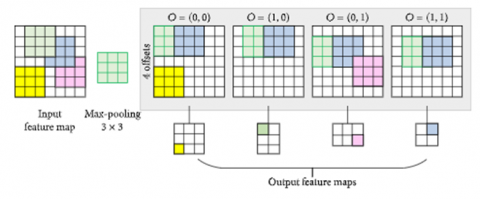
A CNN is composed of one input layer, many hidden layers, and one output layer. Convolutional layers, ReLU (activation function) layers, pooling layers, completely linked layers, and normalisation layers are among the structurally concealed layers. In final step, the completely linked layers are transformed into convolutional layers, which can handle images of any scale, and reshape their parameters, and we use the convolutional network to cope with input images of varying dimensions. This model shows that expanding a sliding window of dimension of the length 6 x 6 on the original picture and assigning the expansion to the FC size yields a 224 × 224 feature calculation detection window in the classifier.
We transform the fully connected layers into convolutional layers and restructure layer settings because to the high computational complexity of the original sliding window approach; so that we can use the fully convolutional network to deal with input images of size 224 x 224 of arbitrary sizes. If we continue without convolution, you will require 224 x 224 x 3 = 100,352 neurons in the input layer, however after convolution, your input vector dimensionality is decreased to 1 x 1 x 1000. This suggests that just 1000 neurons are required in the first layer of a feedforward neural network. The max pooling process is clearly detailed in Figure 2.
Figure 2. Max pooling process
The weights are calculated as
${{W}_{*}}={{\underset{{}}{\mathop \min \sum\limits_{i}^{N}{\left( t_{*}^{i}-\Delta _{*}^{i} \right)}}\,}^{2}}+\lambda {{\left\| {{W}_{{{0}^{\alpha }}}} \right\|}^{2}}+Th$ (1)
where, t is the window size, λ is the feature set identity value and N is the maximum pool sets and Th is the threshold limit of the data records. The medical data records are analysed by considering each tuple and comparing with the training data as
$Rs(m,n)=W+\frac{\partial {{R}_{i}}^{T}}{\partial {{R}_{j}}}+\lambda +\frac{1}{2}mean{{(R)}^{L}}\frac{{{\partial }^{2}}Min({{W}_{m}})}{\partial {{W}^{2}}}$ (2)
Here W is the weights of the record provided, R is the record identity value, ∂ is the data similarity level of the neighbouring pixels. The features considered are dimensionality, size of the dataset, maximum threshold, minimum limit, type of the value, age, smoking habit, gender, RBC, WBC etc.
$m(x,y)=\sqrt{\frac{{{\partial }_{L}}}{{{\partial }_{x}}}\left( {{(i,j)}^{2}} \right)+\frac{{{\partial }_{L}}}{{{\partial }_{y}}}\left( {{(i,j)}^{2}} \right)*\min (Rs)}$ (3)
The characteristics are extracted from the medical records and the features Cf are considered as
$C{{f}_{i,j}}=\sum\limits_{i=1}^{M}{\sum\limits_{j=1}^{N}{L{{n}^{\partial }}+}}Ri(m,n)+\frac{{{R}_{\max }}\times {{R}_{\min }}}{Rs(m,n)}\,\,\,$ (4)
Here, the parameters indicate the feature considered and the variables represent the value in each record in the dataset considered. The values are compared with the neighbouring records and then classification is performed. The medical records are considered by normalizing the values with accurate angle of the records of all sets of a cluster group. The normalization is performed as
$\theta (m,n)={{\tan }^{-1}}\left( \frac{\frac{{{\partial }_{L}}}{{{\partial }_{y}}}(m,n)}{\frac{{{\partial }_{L}}}{{{\partial }_{x}}}(m,n)} \right)$ (5)
For an n-generator system with the normalized measures $N M_{i, j} \in\{1,2, \ldots, n\}$, construct an $\mathrm{n} \times \mathrm{n}$ fuzzy relation matrix FRM as
$FRM=\left[ N{{M}_{ij}} \right],0\le N{{M}_{ij}}\le 1$ (6)
where, NMij indicates the degree of association between generator i and generator j of each record set with group similarity values. Based on the group similarity values, the cluster count cc is prefixed as
$\begin{align} & C{{C}^{(I)}}= \\ & \left[ \lambda {{\sum\limits_{i=1}{FRM(R}}_{i}}) \right]+Th+\min (sim(m(i),n(j)) \\\end{align}$ (7)
λ is the cluster centre of each cluster and the cluster groups labelling is performed to fix the values of each category. The labelling process is performed as
$Ln=\left| {{\lambda }_{ij}}-{{\partial }_{ij}} \right|$
$sim(m,m+1)=\frac{\sum\nolimits_{j=1}^{n}{\partial _{r}^{m}{{m}_{j}}}}{\sum\nolimits_{j=1}^{n}{\lambda _{ij}^{m}}+Ri}$ (8)
$\begin{align} & N= \\ & \frac{1}{Ln}\sum\limits_{i=1}^{n}{\left| C{{C}_{t_{j}^{R}}}-FR{{M}_{i_{avg}^{Th}}} \right|}+\frac{1}{Ln}\sum\limits_{j=1}^{n}{\left| FR{{M}_{i}}-{{R}_{j}} \right|} \\ & +\frac{1}{\lambda }\sum\limits_{i=1}^{n}{\left| \frac{{{\partial }_{L}}}{{{\partial }_{y}}}\left( sim{{(i,j)}^{2}} \right) \right|} \\\end{align}$ (9)
The feature vector FV set that is used for the clustering of medical records is calculated as
$F V(I(i, j))=\int_{i=1}^{L} \operatorname{Ln}(i, j)$$+\int_{j=i}^{L} F R M(i, j)+W$$+\frac{1}{\theta(m, n)} \sum_{i=1}^{L}$$\frac{{{\partial }_{L}}}{{{\partial }_{x}}}\left( {{(i,j)}^{2}} \right)$ (10)
where, $\emptyset$ represents the threshold similarity value.
The degree of consistency afforded by feature subset FS with respect to the equivalence classes and the final feature set is represented as
$\begin{align} & FS{{(I(i,j))}^{T}}\,=\left[ \sum\limits_{i\in U}{Ln(c)(1-Ln(c)} \right] \\ & -\sum\limits_{i\in X}{\left( \frac{Ln{{(x)}^{2}}}{\sum\nolimits_{x\in X}^{N}{Cf{{(x)}^{2}}}}\,+\frac{Ln{{(y)}^{2}}}{\sum\nolimits_{y\in Y}^{M}{Cf{{(y)}^{2}}}}\sum\limits_{i\in U}{Ln(c\left| x)(1-p(c\left| x) \right. \right.} \right)} \\\end{align}$ (11)
where, Cf is the correlation between the summarized components and the external variable, N is the lot of considerations, Ln is the mean association between both the aspects and the external variable.
The proposed feature extraction and selection procedure is implemented in ANACONDA platform. The image entry size 3 x 32 x 3 maps were used for transformation of 3 function maps (RGB) to 6 function maps. The maps input is 3 to 6. Different characteristics are extracted in each feature map, so the picture looks different in each feature map. There are several relations between input layer and convolutionary layer, but weight-sharing parameters are fewer. Image configuration is done by 3 x 3 matrix. A binary classifier predicts either positive or negative results for some feedback.
The performance of the classifier could be:
The figures are normally shown in an uncertainty matrix and the regular measurements to assess a classifier that is obtained in a ratio separate from it. The models are then tested on the originally independent test results using these measurements. This provides us with a proxy to see how widespread the paradigm is.
Precision and recall are two important metrics, calculated as:
Precision $=T P /(T P+F P)$
$\operatorname{Recall}=T P /(T P+F N)$
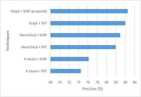
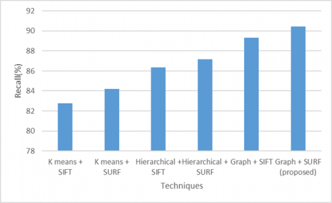
Eventually, with the F1 scores and Intersection Over Union (IoU) the most effective models on each dataset are tested. The Table 1 represents the precision levels comparison of various clustering techniques and Table 2 illustrates the recall comparison of various clustering techniques. The following are described:
$F 1$ Score $=2 *($ Precision $*$ Recall $) /($ Precision $+$ Recall $)$
$I o U=T P /(T P+F P+F N)$
Table 1. Precision comparison of various clustering techniques
|
Techniques |
Precision (%) |
|
K means + SIFT |
74.5126 |
|
K means + SURF |
76.19048 |
|
Hierarchical + SIFT |
81.9632 |
|
Hierarchical + SURF |
82.92683 |
|
Graph + SIFT |
84.0000 |
|
Graph + SURF (proposed) |
84.52735 |
Table 2. Recall comparison of various clustering techniques
|
Techniques |
Recall (%) |
|
K means + SIFT |
82.7536 |
|
K means + SURF |
84.2105 |
|
Hierarchical + SIFT |
86.3589 |
|
Hierarchical + SURF |
87.1794 |
|
Graph + SIFT |
89.3245 |
|
Graph + SURF (proposed) |
90.4568 |
The measure of the related numbers among the retrieved numbers is that of precision. Here Figure 3 represents precision comparison of various clustering techniques. Proposed model performs better compared to existing models in a great extent.
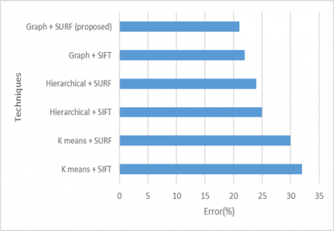
Recall is the percentage of all of usable data that was discovered. Here Figure 4 represents recall comparison of various clustering techniques. Proposed model performs better compared to existing models in a great extent. The Table 3 represents the F-measure comparison of various clustering techniques and Table 4 indicates the error rate comparison of various clustering techniques.
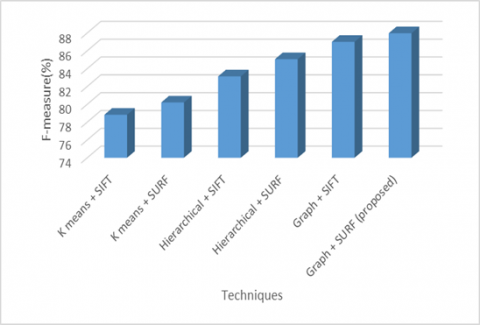
It often referred to as the F1 ranking, it represents the accuracy of a model on a dataset. Most models of knowledge retrieval use the F-score as a measure of complexity. Here Figure 5 represents F-measure comparison of various clustering techniques. Proposed model performs better compared to existing models in a great extent.
Figure 3. Precision comparison of various clustering techniques
Figure 4. Recall comparison of various clustering techniques
Table 3. F-measure comparison of various clustering techniques
|
Techniques |
F-measure (%) |
|
K means + SIFT |
78.8246 |
|
K means + SURF |
80.2005 |
|
Hierarchical + SIFT |
83.1256 |
|
Hierarchical + SURF |
85.0531 |
|
Graph + SIFT |
87.0000 |
|
Graph + SURF (proposed) |
87.9658 |
Table 4. Error comparison of various clustering techniques
|
Techniques/ Metrics |
Error (%) |
|
K means + SIFT |
32.00 |
|
K means + SURF |
30.00 |
|
Hierarchical + SIFT |
25.00 |
|
Hierarchical + SURF |
24.00 |
|
Graph + SIFT |
22.00 |
|
Graph + SURF (proposed) |
21.00 |
Figure 5. F-measure comparison of various clustering techniques
Figure 6. Error comparison of various clustering techniques
Here Figure 6 represents obtained error comparison of various clustering techniques. Proposed model performs gives minimum error so that it gives better performance compared to existing models. The created clusters are depicted in Figure 7.
Figure 7. Different clustering models forms clusters
Table 5. Accuracy comparison of various clustering techniques
|
Techniques |
Accuracy (%) |
|
K means + SIFT |
66.00 |
|
K means + SURF |
68.00 |
|
Hierarchical + SIFT |
75.00 |
|
Hierarchical + SURF |
76.00 |
|
Graph + SIFT |
78.00 |
|
Graph + SURF (proposed) |
79.00 |
Figure 8. Accuracy comparison of various clustering techniques
The correctness of the test results may be considered to be quantified as a percentage of the test outcomes. The ratio of accurate predictions to overall predictions can be accurately be determined. Here Figure 8 and Table 5 represent accuracy comparison of various clustering techniques. Proposed model performs better compared to existing models.
The number of feature maps in the convolutionary neural network built and the number of pairs of convolutions and sample layers characterise the network complexity. We used average pooling and maximum pooling in our model and found better performance than peak pooling for average pooling. We can conclude that with multiple function maps, we can search the image at different locations. As the number of function maps and convolution layers increases beyond a limit, data testing failure begins to slowly increase. If the learning rate is somewhat high, the training error probably increases after many iterations. We conclude that number of hidden-layer units have as much effect as addition of function maps. The number of parameters to be estimated is reduced by the same weight for each map. The relevant features are only considered that improves the system performance. The proposed work considers neural networks to be clustered. To obtain the resulting clusters, the network must be prepared. The network type and size often depend on the data type. This cluster is validated by DB Index or R Square. The analysis for this research can be applied to analyse with the generation of neural networks with the individual feature selection algorithms. The application domain is highly dependent on the use of neural networks. The procedure is determined by the size of the results. In the proposed model, extremely difficult data can also be processed. The precision levels of the proposed model are high than the existing models. In future, feature reduction strategies can be applied on the proposed model to enhance the performance levels and the hidden layers can also be reduced maintaining high accuracy rates.
[1] Kisekka, V., Giboney, J.S. (2018). The effectiveness of health care information technologies: evaluation of trust, security beliefs, and privacy as determinants of health care outcomes. Journal of Medical Internet Research, 20(4): e107. https://doi.org/10.2196/jmir.9014
[2] Zhao, L., Chen, Z., Yang, L.T., Jamal Deen, M., Wang, Z.J. (2019). Deep semantic mapping for heterogeneous multimedia transfer learning using co-occurrence data. ACM Transactions on Multimedia Computing, Communications, and Applications, 15(1s): 1-21. https://doi.org/10.1145/3241055
[3] Zhang, Q., Bai, C., Yang, L.T., Chen, Z., Li, P., Yu, H. (2019). A unified smart Chinese medicine framework for healthcare and medical services. IEEE/ACM Transactions on Computational Biology and Bioinformatics, 18(3): 882-890. https://doi.org/10.1109/TCBB.2019.2914447
[4] Yin, S., Liu, J., Teng, L. (2016). An improved artificial bee colony algorithm for staged search. TELKOMNIKA Telecommunication, Computing, Electronics and Control, 14(3): 1099-1104. http://dx.doi.org/10.12928/telkomnika.v14i3.3609
[5] Liu, T., Yin, S. (2016). An improved particle swarm optimization algorithm used for BP neural network and multimedia course-ware evaluation. Multimedia Tools and Applications, 76(9): 11961-11974. https://doi.org/10.1007/s11042-016-3776-5
[6] Jie, L., Teng, L., Yin, S. (2017). An improved discrete firefly algorithm used for traveling salesman problem. In: Tan Y., Takagi H., Shi Y. (eds) Advances in Swarm Intelligence. ICSI 2017. Lecture Notes in Computer Science, vol 10385. Springer, Cham. https://doi.org/10.1007/978-3-319-61824-1_64
[7] Yin, S.L., Liu, J. (2016). A K-means approach for map-reduce model and social network privacy protection. Journal of Information Hiding and Multimedia Signal Processing, 7(6): 1215-1221.
[8] Li, P., Chen, Z., Yang, L.T., Zhang, Q., Deen, M.J. (2018). Deep convolutional computation model for feature learning on big data in Internet of things. IEEE Transactions on Industrial Informatics, 14(2): 790-798. https://doi.org/10.1109/TII.2017.2739340
[9] Zhao, L., Chen, Z., Yang, Y., Zou, L., Wang, Z.J. (2019). ICFS clustering with multiple representatives for large data. IEEE Transactions on Neural Networks and Learning Systems, 30(3): 728-738. https://doi.org/10.1109/TNNLS.2018.2851979
[10] Gao, J., Li, P., Chen, Z. (2019). A canonical polyadic deep convolutional computation model for big data feature learning in internet of things. Future Generation Computer Systems, 99: 508-516. https://doi.org/10.1016/j.future.2019.04.048
[11] Zhang, Q., Bai, C., Chen, Z., Li, P., Yu, H., Wang, S., Gao, H. (2019). Deep learning models for diagnosing spleen and stomach diseases in smart Chinese medicine with cloud computing. Concurrency and Computation: Practice and Experience, 33(7): 1-1. https://doi.org/10.1002/cpe.5252
[12] Yang, J., Xie, Y., Guo, Y. (2019). Panel data clustering analysis based on composite PCC: A parametric approach. Cluster Computing, 22(S4): 8823-8833. https://doi.org/10.1007/s10586-018-1973-x
[13] Parvin, H., Minaei-Bidgoli, B. (2013). A clustering ensemble framework based on elite selection of weighted clusters. Advances in Data Analysis and Classification, 7(2): 181-208. https://doi.org/10.1007/s11634-013-0130-x
[14] Zhao, L., Chen, Z., Yang, Y., Wang, Z.J., Leung, V.C.M. (2018). Incomplete multi-view clustering via deep semantic mapping. Neurocomputing, 275: 1053-1062. https://doi.org/10.1016/j.neucom.2017.07.016
[15] Zhao, W., Yan, L., Zhang, Y. (2018). Geometric-constrained multi-view image matching method based on semi-global optimization. Geo-spatial Information Science, 21(2): 115-126. https://doi.org/10.1080/10095020.2018.1441754
[16] Li, P., Chen, Z., Yang, L.T., Zhao, L., Zhang, Q. (2017). A privacy-preserving high-order neuro-fuzzy c-means algorithm with cloud computing. Neurocomputing, 256: 82-89. https://doi.org/10.1016/j.neucom.2016.08.135
[17] Meng, Z., Pan, J.S., Kong, L. (2018). Parameters with adaptive learning mechanism (PALM) for the enhancement of differential evolution. Knowledge-Based Systems, 141: 92-112. https://doi.org/10.1016/j.knosys.2017.11.015
[18] Zhang, Q., Yang, L.T., Chen, Z., Li, P. (2017). PPHOPCM: privacy-preserving high-order possibilistic c-means algorithm for big data clustering with cloud computing. IEEE Transactions on Big Data. https://doi.org/10.1109/TBDATA.2017.2701816
[19] Li, J., Ma, T., Tang, M., Shen, W., Jin, Y. (2017). Improved FIFO scheduling algorithm based on fuzzy clustering in cloud computing. Information, 8(1): 1-13. 2017. https://doi.org/10.3390/info8010025
[20] Nogueira, S., Sechidis, K., Brown, G. (2017). On the stability of feature selection algorithms. The Journal of Machine Learning Research, 18(1): 6345-6398.
[21] Song, X., Waitman, L.R., Hu, Y., Yu, A.S., Robins, D., Liu, M. (2019). Robust clinical marker identification for diabetic kidney disease with ensemble feature selection. J Am Med Inf Assoc., 26(3): 242-253. https://doi.org/10.1093/jamia/ocy165
[22] Goh, W.W.B., Wong L. (2016). Evaluating feature-selection stability in next-generation proteomics. J Bioinform Comput Biol., 14(5): 1650029. https://doi.org/10.1142/S0219720016500293
[23] Pes, B. (2019). Ensemble feature selection for high-dimensional data: A stability analysis across multiple domains. Neural Computing and Applications, 32: 5951-5973. https://doi.org/10.1007/s00521-019-04082-3
[24] González, J., Ortega, J., Damas, M., Martín-Smith, P., Gan, J.Q. (2019). A new multi-objective wrapper method for feature selection-accuracy and stability analysis for BCI. Neurocomputing, 333: 407-418. https://doi.org/10.1016/j.neucom.2019.01.017
[25] Ditzler, G, LaBarck, J., Ritchie, J., Rosen, G., Polikar, R. (2017). Extensions to online feature selection using bagging and boosting. IEEE Transactions on Neural Network and Learning Systems, 29(9): 4504-4509. https://doi.org/10.1109/TNNLS.2017.2746107
[26] Chelvan, P.M., Perumal, K. (2017). A comparative analysis of feature selection stability measures. 2017 International Conference on Trends in Electronics and Informatics (ICEI), pp. 124-128. https://doi.org/10.1109/ICOEI.2017.8300901