Jian-Da Wu* | Bo-Yuan Chen | Wen-Jye Shyr | Fan-Yu Shih
© 2021 IIETA. This article is published by IIETA and is licensed under the CC BY 4.0 license (http://creativecommons.org/licenses/by/4.0/).
OPEN ACCESS
The intelligent transportation system is one of the most important constructions of urban modernization. Traffic flow monitoring technology is the most essential information in the intelligent transportation system. With the advancements in instrumentation, computer image processing and communication technology, computerized traffic monitoring technologies have become feasible. This study captures traffic information using surveillance cameras installed at higher locations. The YOLO object detection technology is used to identify vehicle types. The system principle uses image processing and deep convolutional neural networks for object detection training. Vehicle type identification and counting are carried out in this study for straight-line bidirectional roads, and T-shaped and cross-type intersections. A counting line is defined in the vehicle path direction using the object tracking method. The center coordinate of the object moves through the counting line. The number of motorcycles, small vehicles, and large vehicles were counted in different road sections. The actual number of vehicles on the road was compared with the number of vehicles measured by the system. Three separate counting periods were used to define the results using the confusion matrix.
vehicle classification system, convolution neural network, traffic flow, intelligent transportation system
Vehicle detection and classification is an important part of a smart transportation system. The goal is to collect information from vehicles and derive some useful flags such as vehicle speed measurements, traffic density, vehicle counts, traffic congestion lengths, vehicle collisions, average traffic speeds, and vehicle amounts within a period. This information can be used in traffic management to make the traffic flow smoother. In recent years, sensor technology has improved greatly. Using advanced semiconductor technology various sensors have become cheap enough for use in image detection to reduce the manpower and time cost.
Vehicle detection methods include three parts. The first part is the sensor. Sensors include acoustic sensors, magnetometers, accelerometers, ultrasonic and microwave radars and laser scanning [1-6]. The second part is signal processing. For example, the wavelet packet autocorrelation function method [7]. The third part is data processing and analysis such as GPS data for floating cars [8]. The most common traffic flow calculation method is based on intrusive induction which embeds sensors under the road surface. Such a system needs maintenance and regular calibration; thus, producing serious traffic interruption.
Image recognition based on outdoor surveillance cameras is more susceptible to weather, lighting, shadows, etc. than other technologies. However, the image recognition system can provide various advantages, such as not disturbing traffic areas, easy installation and easy modification. Vehicle detection research greatly increased in the past decade supporting the rapid development of intelligent transportation systems [9, 10]. Image processing technology development and the extensive installation of road cameras have facilitated image-based vehicle detection and classification. The most common vehicle image recognition detection method is to use background subtraction for the detection of simple moving objects [11]. For each input traffic image frame, the absolute difference between the generated background model and the current video frame is calculated to extract the vehicle images on the road. To detect the foreground areas of the vehicle, the background modelling process needs to be learned and maintained, such as the Gaussian Mixture Model [12]. Both of the above methods require a stable background for the object to be detected. It is difficult for the program to deal with shadows and the occlusion of large vehicles, which will result in multiple vehicles appearing as a single object. Instant vehicle road detection requires an adaptive non-static background [13].
The continuous improvement in hardware computing power has permitted the rapid development of convolutional neural networks and achieved good results in the computer vision field [14]. At present, the most commonly used methods for object detection are R-CNN series [15, 16], SSD series [17, 18] and YOLO series [19, 20]. The YOLO algorithm was proposed by Redmon and Farhadi [21]. The YOLO algorithm is continuously improved. The YOLOv3 model solves object detection as a regression problem, and uses the K-means clustering method to automatically select the best initial regression for the data set frame. The multi-scale anchor frame concept is used to improve the detection accuracy for small objects [22]. In one step the location and classification of objects are output onto an end-to-end network. This method is one of the fastest algorithms at present.
A better trade-off between speed and accuracy is made in this study. The YOLOv3-SPP model pyramid feature is used as the vehicle detection method [23]. Large buses and large container vehicles are classified as heavy vehicles; small container vehicles and passenger cars, and sport utility vehicles and vans are classified as small cars. Motorcycles are classified into their own separate category. A passenger car equivalent (PCE) provides the vehicle conversion into the reference vehicle [24]. The small passenger car equivalent is the proportion of traffic in the traffic flow compared to small passenger cars under the existing road layout, traffic plan and management measures. For example, a motorcycle is 0.3 small passengers, the small one is a small passenger, and the large one is 1.5 small passengers, etc., to convert traffic flow information into small passenger equivalents. This is very important data for future road construction, traffic signing, and road traffic control.
The convolutional neural network is a multi-level feedforward neural network. The convolutional neural network can automatically learn image features with high nuances, and can be identified on the graph without the function of hand-crafted features. The object detection task is composed mainly of three different algorithms: object localization, feature extraction and image classification. This study uses YOLO object detection that combines the original scattered object detection steps into a single neural network, predicts each bounding box through the features of the entire image, and simultaneously calculates the probability of each bounding box for each class. The object bounding box and the location of the center point are then obtained. YOLO detects objects from the entire image and end-to-end [25], trains and calculations, and also maintains high precision in real-time operations.
The YOLO object detection method is based mainly on the GoogLeNet [26] image classification model. It extracts the input image characteristics from the initial convolutional layer and predicts the probability of the full-connected layer output. Each square is predicted by the convolutional neural network to include the target frame. The YOLO detection method confidence index is the basis for the detection model output. Eq. (1) of the confidence index is as follows:
$\text { Confidence Score } \left.\sigma\left(t_{o}\right)=\operatorname{Pr} \text { (Object }\right) * \text { IoU }_{p r e d}^{\text {truth }}$ (1)
Each bounding box corresponds to a confidence score. If there is no object in the grid cell, the confidence score is zero. If there are objects in the square, the confidence score is the perdition bounding boxes and the real marker IoU value of the bounding boxes. There are two main methods for solving multi-scale problems in the past, one is the image pyramid, and the other is the convolution kernel pyramid. When two different objects are in close proximity, causing the center point of the two objects to share a set of grid cells, the problem of object overlap occurs. In order to solve the problem of overlapping multiple objects in an image, the author proposes an anchors mechanism to introduce anchors of different sizes and different aspect ratios as pre-defined default bounding boxes.
During the object detection process the same area in the image is easily covered by multiple bounding boxes. The non-max suppression algorithm solves this common problem. When bounding box prediction is repeated in object detection, IoU is used to define a threshold value to define the repeated region. A threshold value IoU ≥ 0.5 is the object that we want to focus on. The bounding box datum for all IoU comparisons is then identified, which is the bounding box with the highest probability of prediction in this repeating region. Bounding boxes with the IoU ≥ 0.5 of the base bounding boxes are then discarded. IoU refers to the intersection between the ground-truth bounding boxes and perdition's bounding boxes divided by the union of the two bounding boxes. The IoU calculation is shown in the ground-truth and predicted results shown in Figure 1. The red line is the correct result for the artificial mark. The green line is the result predicted by the algorithm. What IoU has to do is measure the algorithm accuracy in these two results. Therefore, IoU can be used directly as an important indicator of the detection model accuracy.
Figure 1. IoU accuracy calculation
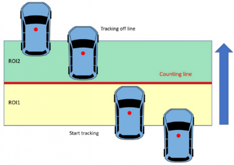
Figure 2. Schematic diagram of Region of Interest
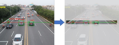
Figure 3. Image tracking area after image processing
Because the image detection process will get a new object list every time an object is detected in the object frame, the objects in the upper and lower frames cannot determine whether it is the same vehicle if the training weight is insufficient. In the travel direction a single object will result in multiple calculations. In order to avoid double counting it must be solved by object tracking. In the image processing procedure, the images of some objects can only be processed and analyzed through region of interest (ROI). The image ROI often outlines the areas to be processed in the form of boxes, circles, ellipses, irregular polygons, and the like. A part of the image is separated from the area for processing, which reduces the image processing analysis workload, improves the precision and reduces the processing time.
In the middle of the lane image, a count line is drawn perpendicular to the lane in the lane image. The thickness is 1 pixel. A thick line of 20 pixels is expanded on the upper and lower sides of the count line. The two thick lines cover the ROI1 and ROI2 regions of interest. The tracking action is started when a vehicle center point position enters ROI1. If the center point of the object enters ROI2 through the counting line in the next frame, the vehicle direction is obtained through the upper and lower frames and the number of vehicles in that direction is increased by one, as shown in Figure 2. It shows a schematic diagram of the area of interest. It is not necessary to calculate the vehicle flow and direction for the entire image during object tracking. Just add the drawn line segment and ROI area to the hidden layer and then judge and calculate when a vehicle passes this line or this area. After the center point of the object passes through the traced area drawn in the front, the number of objects is added. Figure 3 shows the image processing detection area after image processing.
Table 1. Equipment and operating environment
|
OS |
Ubuntu 16.04 LTS |
|
CPU |
Intel Core i7-7700 4.2GHz |
|
GPU |
GeForce GTX1080Ti 11G |
|
RAM |
64 GB |
|
Camera |
Canon EOS M50 |
|
Camera lens |
EF-M 11-22mm f/4-5.6 IS STM |
|
Video specification |
1920*1080/60FPS |
Figure 4. Camera installation diagram
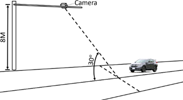
The development environment for the entire identification system used Python language. Python is an object-oriented high-level programming language and a literal translation language. The system hardware equipment mainly uses the GTX 1080Ti display card as the main core of the whole system operation. The environment and operating system mainly used for data collection and feature engineering are shown in Table 1. This study carried out scorpion type classification and the vehicle counting system. Traffic flow filming must be carried out in locations that are conducive to the recording of motorcycles, cars and heavy vehicles. In consideration of the need to photograph motorcycles, the traffic is filmed at a height of about eight meters in the urban area. A straight-line bidirectional road film is taken on two road sections. As shown in Figure 4, the relevant position for the vehicles and camera frame is shown.
The system architecture of this experiment is to set up a camera on an overpass to take images of three different road sections as a database. The three road types recorded were straight-line bidirectional road, T-shaped intersection and cross-type intersection. This section of the shooting angle is divided into two types: camera shoots north and camera shoots south. There are 12 videos on straight-line bidirectional road, each videotape takes about two minutes, codenamed A1-A12, A1-A6 are taken by the camera to the north, A7-A12 are taken by the camera to the south, A1-A3 is used as a training sample for CNN, internal testing is used for identification, A4-A12 is an external test.
Figure 5. Video classification process
The T-shaped road is located at the intersection of the road. Two videos were shot on T-shaped road, codenamed B1 and B2. B1 is used as the training sample for CNN. B2 is used for external testing. The cross-type road is located at the intersection of highway expressway and county road. Two videos were taken on the cross-type intersection, codenamed C1 and C2. C1 is used as a training sample for CNN, and C2 is an external test. The three road types used five videos as training samples, as summarized in Figure 5. The five videos codenamed A1-A3 and B1 and C1 output 10,003 pictures for cars, 673 pictures for heavy vehicles, and 6,185 pictures for motorbike. A total of 16,861 pictures were used for training. The training sample for this study is shown in Table 2.
Table 2. Number of training samples
|
Sample category |
Number of samples |
|
Car |
10,003 |
|
Heavy vehicles |
673 |
|
Motorbike |
6,185 |
|
Total |
16,861 |
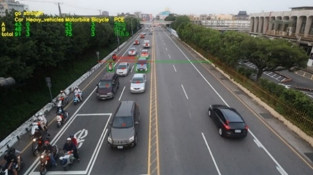
In feature engineering, 8 videos are used as training samples. The video is used to capture 2 pictures in 1 second. The rectangle frame is used to frame the boundary of the object. After training using CNN, the system will obtain the positional data of the object's bounding box and the object category confidence in the rectangular box, and output a weight. After completing the training, the traffic flow in the video is randomized, the trained weight model input to classify and mark the objects, and finally the trained model is evaluated to obtain the optimization weight. The system flow chart is indicated in Figure 6. From the incremental decrease in the center point of the vehicle images in the upper and lower frames, the number and direction of vehicles passing the count line are determined as shown in Figure 7, the external test straight-line bidirectional road movement detection and counting result map. Figure 8 is the external test T-shaped intersection mobile detection and counting result graph. Figure 9 is a diagram showing the motion detection and counting results for the external test cross-type intersection.
Figure 6. System flow chart
Figure 7. Straight-line bidirectional road counting result
Figure 8. T-shaped intersection count result
Figure 9. Cross-type intersection result
This experiment recorded videos on straight-line bidirectional roads, T-shaped intersections and cross-type intersection. Three experimental conditions were recorded in 1 to 2 minutes of video and divided into two parts for testing, the first part is internal testing. The internal test is to sample five videos codenamed A1-A3 and B1 and C1 for training, and obtain the weight after training, and then use this weight to test the five videos with the classification and counting system of this study. The second part is the external test. The external test is in the un-retrained samples of the video. After the training weights, the external video data was tested with the classification and counting system of this study. Eleven films codenamed A4-A12 and B2 and C2 for external testing. The actual number of vehicles on the road was compared with the number of vehicles measured by the system. Three counting results were obtained using the Confusion Matrix, which is defined as shown in Eqns. (2) to (4) [27].
$P R=\frac{T P}{T P+F P}$ (2)
$\mathrm{RR}=\frac{T P}{T P+F N}$ (3)
$F_{m}=\frac{2 \cdot P R \cdot R R}{P R+R R}$ (4)
The number of positive examples detected correctly is called (True Positive, TP). The number of positive examples detected as positive examples is called (False Positive, FP), and the number of positive examples detected as negative examples is called (False Negative, FN). The precision rate (PR) is the ratio of the correct number of parameters retrieved by the system to the total number of parameters retrieved by the system. The precision rate is a measure ranging between 0 and 1 that indicates the detection accuracy rate relative to ground truth. The recall rate (RR) is the correct number of turns retrieved and the actual total number of vehicles. The recall rate is also a measure ranging between 0 and 1 that can be interpreted as the converse of the omission error.
The ratio of $F_{m}$ (F-measure, $F_{m}$ ) is a weighted harmonic average that takes into account both the precision and the recall. This is applied to an evaluation of the retrieval system effectiveness and can also be used to compare the difference in performance between different technologies or systems. The system detection and counting results for three vehicle internal testing classes under the videos codename A1-A3 are relatively stable. Table 3 shows the average counting results for three vehicle external testing classes under the videos codename A4-A12. The $F_{m}$ metric of 9 videos are all above 97%.
Table 3. Results of external test in straight-line bidirectional roads
|
A4-A12 straight-line bidirectional road |
||||||
|
Video |
TP |
FP |
FN |
PR (%) |
RR (%) |
Fm (%) |
|
A4 |
165 |
3 |
0 |
98.21 |
100 |
99.1 |
|
A5 |
177 |
6 |
1 |
96.72 |
99.44 |
98.06 |
|
A6 |
197 |
7 |
0 |
96.57 |
100 |
98.25 |
|
A7 |
167 |
5 |
0 |
97.09 |
100 |
98.53 |
|
A8 |
176 |
3 |
0 |
98.32 |
100 |
99.15 |
|
A9 |
176 |
7 |
2 |
96.17 |
98.9 |
97.51 |
|
A10 |
59 |
1 |
0 |
98.33 |
100 |
99.16 |
|
A11 |
185 |
0 |
1 |
100 |
99.46 |
99.73 |
|
A12 |
133 |
0 |
0 |
100 |
100 |
100 |
|
Total |
1435 |
32 |
4 |
97.82 |
99.72 |
98.76 |
Table 4. Results of external test in T-shaped intersection roads
|
B2 T-shaped intersection |
|||||||
|
Lane |
vehicle classification |
TP |
FP |
FN |
PR (%) |
RR (%) |
Fm (%) |
|
A |
car |
24 |
0 |
0 |
100 |
100 |
100 |
|
heavy vehicles |
2 |
0 |
0 |
100 |
100 |
100 |
|
|
motorbike |
8 |
0 |
1 |
100 |
88.89 |
94.12 |
|
|
B |
car |
30 |
3 |
0 |
90.91 |
100 |
95.24 |
|
heavy vehicles |
0 |
0 |
0 |
100 |
100 |
100 |
|
|
motorbike |
7 |
1 |
0 |
87.50 |
100 |
93.33 |
|
|
C |
car |
1 |
0 |
0 |
100 |
100 |
100 |
|
heavy vehicles |
0 |
0 |
0 |
100 |
100 |
100 |
|
|
motorbike |
0 |
0 |
0 |
100 |
100 |
100 |
|
|
Total |
72 |
4 |
1 |
94.74 |
98.63 |
96.64 |
|
Table 5. Results of external test in cross-type intersection
|
Lane |
vehicle classification |
TP |
FP |
FN |
PR (%) |
RR (%) |
Fm (%) |
|
A |
car |
14 |
0 |
0 |
100 |
100 |
100 |
|
heavy vehicles |
1 |
0 |
0 |
100 |
100 |
100 |
|
|
motorbike |
1 |
0 |
0 |
100 |
100 |
100 |
|
|
B |
car |
14 |
0 |
2 |
100 |
87.5 |
93.33 |
|
heavy vehicles |
0 |
0 |
0 |
100 |
100 |
100 |
|
|
motorbike |
3 |
0 |
0 |
100 |
100 |
100 |
|
|
C |
car |
25 |
0 |
2 |
100 |
92.59 |
96.15 |
|
heavy vehicles |
2 |
0 |
0 |
100 |
100 |
100 |
|
|
motorbike |
0 |
0 |
0 |
100 |
100 |
100 |
|
|
D |
car |
1 |
0 |
0 |
100 |
100 |
100 |
|
heavy vehicles |
0 |
0 |
0 |
100 |
100 |
100 |
|
|
motorbike |
2 |
0 |
0 |
100 |
100 |
100 |
|
|
Total |
63 |
0 |
4 |
100 |
94.03 |
96.92 |
Table 4 shows the average counting results for three vehicle classes in the T-shaped intersection external testing under the videos codename B2. It can be seen that the system detection count results in 4 over counts and 1 undercount in 72 vehicles. It has been observed that due to the complexity of the road environment and the angle of recording, small objects are easily covered by large vehicles during detection. This may result in vehicle leakage. The case of multiple calculations occurs when an object passes through the zebra crossing and the background is complicated by the black and white stripes of the zebra crossing. When the object is detected, a jump in the object frame leads to multiple calculations. The counting system will then have multiple counts and misses. The rate and recall rate and Fm metrics are both decreased, but the precision rate remains at 94.74%. The recall rate remains at 98.63%. The Fm metric also maintained good performance above 96.64%.
Table 5 shows the average counting results for three vehicle classes in the cross-type intersection external test under the videos codename C2. C1 can be seen that in the 55 vehicles five cars are missing from counting system. It was observed that the poles, wires and traffic lights created shadows on the road due to the sun, which caused the system to calculate higher leakage than the first two sections because of the intersection. This traffic environment was shot with an aerial camera. The image is easy to shake up and down slightly, and the counting line is fixed in the image. It is easy to generate multiple counts when shaking, so that the recall rate is maintained at 94.03%. In the case of a missed vehicle, the precision is only maintained at 100%. After the precision and recall average the Fm metric is 96.92%.
Table 6. Average counting results for three classes of vehicle in index by road type
|
roads classification |
TP |
FP |
FN |
PR (%) |
RR (%) |
Fm(%) |
|
straight line |
1944 |
32 |
10 |
98.38 |
99.49 |
98.93 |
|
T-shaped |
137 |
4 |
1 |
97.16 |
99.28 |
98.21 |
|
cross-type |
118 |
1 |
5 |
99.16 |
95.93 |
97.52 |
|
Total |
2199 |
37 |
16 |
98.35 |
99.28 |
98.81 |
Table 6 shows the average counting results for three vehicle classes in the videos codename A1-A12, B1-B2 and C1-C2 index by road type. It can be seen straight line bidirectional road that in the 1944 vehicles, 32 vehicles are extra and 10 vehicles are missing from counting system. After the precision and recall average the Fm metric is 98.93%. In the T-shaped intersection 137 vehicles, 32 vehicles are extra and 10 vehicles are missing from counting system. After the precision and recall average the Fm metric is 98.21%. In the cross-type intersection 118 vehicles, 1 vehicle is extra and 5 vehicles are missing from counting system. After the precision and recall average the Fm metric is 97.52%. In the three categories of roads, heavy vehicles and motorbike, the heavy vehicles do not have over counting and undercounting. According to observations of three roads, more complex routes and backgrounds are prone to systematic misjudgments. The detection performance of four models is summarized in Table 7. It can be clearly seen from the results that Yolov3-SPP has the best recognition rate effect in three road conditions of present system.
Table 7. Detection performance of four models
|
|
mAP (%) |
||
|
Straight-line |
T-shaped |
Cross-type |
|
|
yolov3 |
88.3 |
87.2 |
84.3 |
|
yolov3-tiny |
88.5 |
88.3 |
84.6 |
|
yolov4 |
90.2 |
89.4 |
89.5 |
|
yolov3-spp |
98.8 |
96.6 |
98.8 |
This study proposed a vehicle motion detection and classification counting system using a convolutional neural network to classify motorcycles, small cars and large vehicles in different categories. The image processing technology used in this system completes object tracking and the object tracking system classifies and counts the vehicles according to the input weight and the object category identification parameters. From the experimental results using these three types of defects, it was found that the objects will be in shadows, the zebra crossing, the vehicle stays on the counting line, and large vehicles will cover small vehicles. The system will have multiple calculations and missed measures, so the system will have multiple counts and misses. In completes the effectiveness evaluation for the entire system and road capacity estimation, PCE provides a mechanism for converting vehicles into vehicle types. The small passenger equivalent is a very important data for the future road construction, the setting of traffic signs and the formulation of road traffic control. In the future, system stability will be continuously improved. With the advancement of GPUs and learning algorithm the accuracy and timeliness can be significantly improved in the future. The experimental results show that this method feasible and is expected to be applied continuously in the future of smart transportation systems.
The study was supported by the Ministry of Science and Technology of Taiwan, Republic of China, under project number MOST 109-2221-E-018-013.
[1] Mimbela, L.E.Y., Klein, L.A. (2000). A summary of vehicle detection and surveillance technologies used in intelligent transportation systems. Vehicle Detector Clearinghouse, Las Cruces, New Mexico, USA.
[2] Barbagli, B., Bencini, L., Magrini, I., Manes, G. (2011). A traffic monitoring and queue detection system based on an acoustic sensor network. International Journal on Advances in Networks and Services, 4(1&2): 27-37. http://doi.org/10.1.1.685.7934
[3] Zhang, L., Wang, R., Cui, L. (2011). Real-time traffic monitoring with magnetic sensor networks. Journal of Information Science and Engineering, 27(4): 1473-1486. https://doi.org/10.1688/JISE.2011.27.4.17
[4] Lombaert, G., Degrande, G. (2003). The experimental validation of a numerical model for the prediction of the vibrations in the free field produced by road traffic. Journal of Sound and Vibration, 262(2): 309-331. https://doi.org/10.1016/S0022-460X(02)01048-9
[5] Jo, Y., Jung, I. (2014). Analysis of vehicle detection with WSN-based ultrasonic sensors. Sensors, 14(8): 14050-14069. https://doi.org/10.3390/s140814050
[6] Tian, Y., Liu, H., Furukawa, T. (2017). Reliable infrastructural urban traffic monitoring via Lidar and camera fusion. SAE International Journal of Passenger Cars - Electronic and Electrical Systems, 10(1): 173-180. https://doi.org/10.4271/2017-01-0083
[7] Jiang, X., Adeli, H. (2004). Wavelet packet‐autocorrelation function method for traffic flow pattern analysis. Computer-Aided Civil and Infrastructure Engineering, 19(5): 324-337. https://doi.org/10.1111/j.1467-8667.2004.00360.x
[8] Zhou, X., Wang, W., Yu, L. (2013). Traffic flow analysis and prediction based on GPS data of floating cars. In: Lu W., Cai G., Liu W., Xing W. (eds) Proceedings of the 2012 International Conference on Information Technology and Software Engineering. Lecture Notes in Electrical Engineering, 210: 497-508. https://doi.org/10.1007/978-3-642-34528-9_51
[9] Liu, Y., Tian, B., Chen, S., Zhu, F., Wang, K. (2013). A survey of vision-based vehicle detection and tracking techniques in ITS. Proceedings of 2013 IEEE International Conference on Vehicular Electronics and Safety, Dongguan, China, pp. 72-77. https://doi.org/10.1109/ICVES.2013.6619606
[10] Sivaraman, S., Trivedi, M.M. (2013). Looking at vehicles on the road: A survey of vision-based vehicle detection, tracking, and behavior analysis. IEEE Transactions on Intelligent Transportation Systems, 14(4): 1773-1795. https://doi.org/10.1109/TITS.2013.2266661
[11] Gupte, S., Masoud, O., Martin, R.F.K., Papanikolopoulos, N.P. (2002). Detection and classification of vehicles. IEEE Transactions on Intelligent Transportation Systems, 3(1): 37-47. https://doi.org/10.1109/6979.994794
[12] Stauffer C., Grimson, W.E.L. (1999). Adaptive background mixture models for real-time tracking. Proceedings 1999 IEEE Computer Society Conference on Computer Vision and Pattern Recognition (Cat. No PR00149), Fort Collins, CO, USA, 2: 246-252. https://doi.org/10.1109/CVPR.1999.784637
[13] Sullivan, G.D., Baker, K.D., Worrall, A.D., Attwood, C.I., Remagnino, P.M. (1997). Model-based vehicle detection and classification using orthographic approximations. Image and Vision Computing, 15(8): 649-654. https://doi.org/10.1016/S0262-8856(97)00009-7
[14] Lecun, Y., Bottou, L., Bengio, Y., Haffner, P. (1998). Gradient-based learning applied to document recognition. Proceedings of the IEEE, 86(11): 2278-2324. https://doi.org/10.1109/5.726791
[15] Girshick, R., Donahue, J., Darrell T., Malik, J. (2014). Rich feature hierarchies for accurate object detection and semantic segmentation. 2014 IEEE Conference on Computer Vision and Pattern Recognition, Columbus, OH, USA, pp. 580-587. https://doi.org/10.1109/CVPR.2014.81
[16] He, K., Gkioxari, G., Dollár P., Girshick, R. (2017). Mask R-CNN. 2017 IEEE International Conference on Computer Vision (ICCV), Venice, Italy, pp. 2980-2988. https://doi.org/10.1109/ICCV.2017.322
[17] Liu, W., Anguelov, D., Erhan, D., Szegedy, C., Reed, S., Fu, C.Y., Berg, A.C. (2016). SSD: Single shot multibox detector. In European Conference on Computer Vision, 9905: 21-37. https://doi.org/10.1007/978-3-319-46448-0_2
[18] Fu, C.Y., Liu, W., Ranga, A., Tyagi, A., Berg, A.C. (2017). DSSD: Deconvolutional single shot detector. https://arxiv.org/abs/1701.06659
[19] Redmon, J., Divvala, S., Girshick, R., Farhadi, A. (2016). You only look once: Unified, real-time object detection. 2016 IEEE Conference on Computer Vision and Pattern Recognition (CVPR), Las Vegas, NV, USA, pp. 779-788. https://doi.org/10.1109/CVPR.2016.91
[20] Redmon, J., Farhadi, A. (2017). YOLO9000: Better, faster, stronger. 2017 IEEE Conference on Computer Vision and Pattern Recognition (CVPR), Honolulu, HI, USA, pp. 6517-6525. https://doi.org/10.1109/CVPR.2017.690
[21] Redmon, J., Farhadi, A. (2018). Yolov3: An incremental improvement. https://arxiv.org/abs/1804.02767.
[22] Zhu, C., Tao, R., Luu, K., Savvides, M. (2018). Seeing small faces from robust anchor's perspective. 2018 IEEE/CVF Conference on Computer Vision and Pattern Recognition, Salt Lake City, UT, USA, pp. 5127-5136. https://doi.org/10.1109/CVPR.2018.00538
[23] He, K., Zhang, X., Ren, S., Sun, J. (2015). Spatial pyramid pooling in deep convolutional networks for visual recognition. IEEE Transactions on Pattern Analysis and Machine Intelligence, 37(9): 1904-1916. https://doi.org/10.1109/TPAMI.2015.2389824
[24] Institute of Transportation. (2011). Highway Capacity Manual in Taiwan. Report No. 100-132-1299. Ministry of Transportation and Communication, Taiwan.
[25] Huang, L., Yang, Y., Deng, Y., Yu, Y. (2015). DenseBox: Unifying landmark localization with end to end object detection. https://arxiv.org/abs/1509.04874v3
[26] Szegedy, C., Liu, W., Jia, Y., Sermanet, P., Reed, S., Anguelov, D., Erhan, D., Vanhoucke, V., Rabinovich, A. (2015). Going deeper with convolutions. 2015 IEEE Conference on Computer Vision and Pattern Recognition (CVPR), Boston, MA, USA, pp. 1-9. https://doi.org/10.1109/CVPR.2015.7298594
[27] Niu, X. (2006). A semi-automatic framework for highway extraction and vehicle detection based on a geometric deformable model. ISPRS Journal of Photogrammetry and Remote Sensing, 61(3-4): 170-186. https://doi.org/10.1016/j.isprsjprs.2006.08.004