Peng Xue* | Changhong Jiang | Huanli Pang
© 2021 IIETA. This article is published by IIETA and is licensed under the CC BY 4.0 license (http://creativecommons.org/licenses/by/4.0/).
OPEN ACCESS
Machine vision is a promising technique to promote intelligent production. It strikes a balance between product quality and production efficiency. However, the existing metal surface defect detection algorithms are too general, and deviate from electrical production equipment in the level of response time to the target image. To address the two problems, this paper designs a detection algorithm for various types of metal surface defects based on image processing. Firstly, each metal surface image was preprocessed through average graying and nonlocal means filtering. Next, the principle of the composite model scale expansion was explained, and an improved EfficientNet was constructed to classify metal surface defects, which couples spatial attention mechanism. Finally, the backbone network of the single shot multi-box detector (SSD) network was improved, and used to fuse the features of the target image. The proposed model was proved effective through experiments.
image processing, metal surface, defect detection, EfficientNet
Despite the rapid progress of detection technology, manual quality inspection is still widely used among small and medium-sized enterprises (SMEs) [1-4]. However, it is difficult to visually identify the surface defects on metals. Manual quality inspection alone cannot even ensure the quality stability and consistency of metal products in the same batch, and face relatively high false positive (FP) and false negative (FN) [5-9]. Machine vision is a promising technique to promote intelligent production. It strikes a balance between product quality and production efficiency. However, many technical problems need to be overcome to detect metal surface defects. For example, the detection effect varies with the shapes and causes of metal surface defects [10-13].
One of the key goals of Industry 4.0 and digital production is to support faster, cleaner, and increasingly customizable manufacturing. Di Cataldo et al. [14] integrated advanced visual sensing technology into industrial robot systems, and realized the real-time quality monitoring and flow optimization of massive field data, using multiple time scales and resolutions. To improve the sensitivity of defect detection, Sun et al. [15] mainly adopted two techniques, namely, segmentation of running cycle, and integration between physical and mathematical models. The results on test data show that the adopted techniques can display whether the target robot is qualified or not, and guide the repair of any defect being detected. To detect rare defects, Gutierrez et al. [16] proposed a texture scanning and generation method to render the small defects (e.g., extruding textures and small holes) of metal parts, and evaluated the quality of generated images by training the deep learning (DL) network, and testing on the actual data from the manufacturer. Traditional defect detection algorithms have difficulty in detecting the defects with large shape changes, identifying the defects with massive changes, and locating defects with a high accuracy. To overcome the difficulty, Liu et al. [17] put forward a visual defect detection framework based on convolutional neural network (CNN), and mitigated the above three problems by introducing three modules, namely, deformable convolution module, balanced feature generation module, and cascade header module. Lin H.I. and Lin, P.Y. [18] designed a composite evaluation metric for the image quality of image dataset, and applied it to train the defect detection model. Hu et al. [19] presented a generative adversarial network with the relative average discriminator, which is driven by dual attention mechanisms, to generate high-quality defect images. The network provides a desired solution to the lack of samples and imbalanced classes in the surface defect dataset of metal workpieces in industrial production. Zhou et al. [20] created a metal surface defect detection algorithm based on machine vision: the improved binary empirical mode decomposition (BEMD) algorithm was adopted to filter the complex textures on metal surface, thereby extracting the initial surface defects; meanwhile, the effective information of defects is preserved as much as possible. The performance of the defect detection algorithm was demonstrated through experiments.
The existing metal surface defect detection algorithms are too general for the small defects on the surface of metal workpieces, and deviate from electrical production equipment in the level of response time to the target image. To solve the problems, this paper designs a novel detection algorithm for various types of metal surface defects. Section 2 provides a preprocessing method for metal surface images, which includes average graying and nonlocal means filtering. Section 3 expounds on the principle of the composite model scale expansion, and constructs an improved EfficientNet to classify metal surface defects, which couples spatial attention mechanism. Section 4 takes the EfficientNet with spatial attention mechanism as the backbone network of single shot multi-box detector (SSD) network, and applied it to fuse the features of the target image. The proposed model was proved valid through experiments.
Component method, maximum method, average method and weighted average method are the most common image graying approaches. This paper chooses the commonly used average method to gray the collected metal surface defect images. Similar to the maximum method, the average method defines the gray value of an image pixel as the mean brightness of the three components: red (R), green (G), and blue (B):
$HD\left( i,j \right)=\frac{R\left( i,j \right)+G\left( i,j \right)+B\left( i,j \right)}{3}$ (1)
This paper aims to detect different types of metal surface defects. The detection results might be affected by any slight noise produced in image transmission. Here, the target image is processed by nonlocal average filtering, which can denoise the redundant information that are prevalent in natural images.
Unlike the traditional denoising method, the nonlocal average filtering algorithm removes the noises of the entire image, and searches for the areas in the target image that are similar to defect templates, using each image block as the unit. After the search, the similar areas are averaged. This filtering algorithm can effectively eliminate the Gaussian noise in the image. Let NEa be the neighborhood of pixel a in the target image, i.e., the search area of pixel a; q(b) be the noisy original target image; θ(a, b) be the weight of the similarity between pixels a and b in the image. Then, the nonlocal average filtering can be expressed as:
$\tilde{w}\left( a \right)=\sum\limits_{b\in NE}{\theta \left( a,b \right)q\left( b \right)}$ (2)
where, θ(a, b) falls in the following range:
$\theta \left( a,b \right)\in \left( 0,+\infty \right)\text{ and}\sum\limits_{b\in NE}{\theta \left( a,b \right)}=1,\forall a\in NE,b\in N{{E}_{a}}$ (3)
Formula (3) shows the value of θ(a, b) must be greater than zero, and all the weights should add up to 1. Let EU(a, b) be the Gaussian weighted Euclidean distance between the neighborhoods of pixels a and b. Then, θ(a, b) can be further derived from EU(a, b):
$\theta \left( a,b \right)=\frac{1}{m\left( a \right)}exp\left( \frac{EU\left( a,b \right)}{{{g}^{2}}} \right)$ (4)
Let ε be a positive standard deviation of Gaussian kernel. Then, EU(a, b) can be calculated by:
$EU\left( a,b \right)=\left\| Q\left( a \right)-Q\left( b \right) \right\|_{2,\varepsilon }^{2}$ (5)
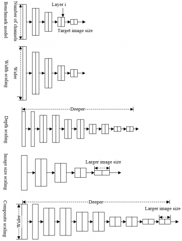
Figure 1. Illustration of composite model scale expansion method
Figure 1 illustrates composite model scale expansion method. The benchmark model was compared with four mesoscale expansion methods, including width scaling, depth scaling, image size scaling, and composite scaling. The depth, width, and input resolution of EfficientNet can be weighed based on a unified proportionality factor, that is, the three parameters can be balanced in the same CNN. Let N be the CNN; Bi=Hi(Ai) be the i-th convolutional layer of the network; Ai and Bi be the three-dimensional (3D) input and output tensors of the image, respectively. Then, the CNN M composed of only 1 convolutional layer can be expressed as:
$M={{H}_{l}}\otimes ...\otimes {{H}_{2}}\otimes {{H}_{1}}\left( {{A}_{1}} \right)={{\Gamma }_{j=1...l}}{{H}_{j}}\left( {{A}_{1}} \right)$ (6)
However, actual image processing networks all adopt multiple identical convolutional layers. Here, the identical convolutional layers are considered as a stage, whose number is i (i=1, 2, …, r). Let <Fi, Ui, Di> be the dimensions of the 3D input tensor Ai of the i-th convolutional layer image, where Fi and Ui are the spatial dimensions of the feature map, and Di is the channel dimension. Let HKii be the component of the i-th convolutional layer Hi repeated Ki times. Then, the CNN M can be expressed as:
$M=\underset{i-1...r}{\mathop{\Gamma }}\,H_{i}^{{{K}_{i}}}\left( {{A}_{\left\langle {{F}_{i}},{{U}_{i}},{{D}_{i}} \right\rangle }} \right)$ (7)
The image space can be reduced by determining Hi in EfficientNet algorithm, that is, the detection accuracy of defects can be maximized under a poor computing ability of hardware equipment by scaling each block evenly in three dimensions by a constant proportion. Let c, u, and s be the width coefficient, depth coefficient, and image resolution coefficient of the neural network, respectively. The objective function of accuracy rate (AR) optimization can be given by:
$\begin{align} & ma{{x}_{c,u,s}}AR\left( M\left( c,u,s \right) \right) \\ & s.t.\ M\left( c,u,s \right)=\underset{i-1...r}{\mathop{\Gamma }}\,H_{i}^{c\cdot {{{\dot{K}}}_{i}}}\left( {{A}_{\left\langle s\cdot {{{\dot{F}}}_{i}},s\cdot {{{\dot{U}}}_{i}},s\cdot {{{\dot{D}}}_{i}} \right\rangle }} \right) \\ & ME \left( M \right)\le TA\_ME \\ & FL\left( M \right)\le TA\_ FL \\ \end{align}$ (8)
where, ME is the target memory limit; FL is the floating-point operations per second (FLOPS) limit. To optimize the defect detection effect, this paper adopts composite scaling method to proportionally scale c, u, and s in EfficientNet, striking a balance between the three. The first step is to determine the constrained optimal parameters δ, ξ and λ that measure the proportions of c, u, and s. Since c and s have a square relationship with network computing load, while u and s do not have such a relationship, square processing was only implemented on the constraints of ξ and λ.
This paper introduces parameter ψ, which satisfies all three dimensions, to optimize the balance between c, u, and s. To facilitate FLOPs calculation and minimize the computing load of the neural network in the search of optimal solution, the values of the three coefficients should be constrained at the same time: δ2.ξ2.λ2≈2 and δ≥1, ξ≥1, and λ≥1. The specific constraints can be expressed as:
$\begin{align} & DE: c={{\delta }^{\psi }} \\ & WI:u={{\xi }^{\psi }} \\ & RE: s={{\lambda }^{\psi }} \\ & s.t.{{\delta }^{2}}\cdot {{\xi }^{2}}\cdot {{\lambda }^{2}}\approx 2\text{ }\delta \ge 1,\xi \ge 1,\lambda \ge 1 \\ \end{align}$ (9)
where, DE, WI, and RE are the constraints on width, depth, and image resolution, respectively. As shown in formula (9), δ, ξ, λ, and ψ are a set of constants and a constant term found by the neural network.
Image convolution, a local operation, pays insufficient attention to the input target image. By introducing the computationally-efficient spatial attention mechanism, this paper optimizes EfficientNet algorithm to increase the projected area of each pixel of the feature map outputted by each neural network layer onto the original image, aiming to improve model performance.
Figure 2 illustrates the structure of spatial attention module. This paper firstly transforms the feature map with three convolutional layers (kernel size: 1×1). The transformation function can be expressed as:
$\left\{ \begin{matrix} x\left( a \right)={{\omega }_{1}}\cdot a \\ y\left( a \right)={{\omega }_{2}}\cdot a \\ z\left( a \right)={{\omega }_{3}}\cdot a \\ \end{matrix} \right.$ (10)
To facilitate the next operation, the matrices x(a) and y(a) obtained through the transformation of the convolutional layer need dimensional variation. The dimensionally-changed matrices were then multiplied with each other to obtain a feature map of the size UF×UF. Then, the spatial attention map can be further generated by softmax function:
${{R}_{v,t}}=\frac{exp\left( x{{\left( {{a}_{t}} \right)}^{T}}\cdot y\left( {{a}_{v}} \right) \right)}{\sum\nolimits_{l=1}^{UF}{exp\left( x{{\left( {{a}_{l}} \right)}^{T}}\cdot y\left( {{a}_{v}} \right) \right)}}$ (11)
where, Rv-t is the relationship between pixels v and t on the feature map. The spatial attention could be composed of Rv-t. Feature fusion is needed to obtain the feature map after the spatial attention transform. Using the convolutional layer with the kernel size of 1×1, matrix z(a) can be obtained. The feature fusion map can be obtained by multiplying matrix z(a) with Rv-t. Then, a coefficient ξ was introduced to multiply with the feature fusion map, and then superposed on the original feature map av:
$O{{U}_{v}}={{a}_{v}}+\xi \cdot \left( \sum\nolimits_{t=1}^{UF}{{{R}_{v-t}}\cdot z\left( {{a}_{v}} \right)} \right)$ (12)
where, ξ is initialized as zero. The ξ value should be gradually increased to improve the effectiveness of attention on features. In theory, the additional spatial attention module is stochastic, and capable of processing channels and matrix information at the same time.
Figure 2. Structure of spatial attention module
Table 1 shows the structure of the EfficientNet with spatial attention mechanism, where Conv1 and Conv6 represent the scale expansion ratios of 1 and 6, respectively.
This paper takes the EfficientNet algorithm coupled with spatial attention mechanism as the backbone network of SSD network, and fuses the features of the target image. In this way, the network becomes more capable of expressing and detecting the defects in the image.
4.1 Model construction
The SSD network, as a single-stage target detection network, can detect defects quickly and accurately, and meet the requirements of real-time detection. The target detection effect of SSD network is better than you only look once (YOLO) and Faster Region-Based CNN (R-CNN).
To enhance feature extraction ability, the SSD network with multiscale feature maps has a customized convolutional layer after each convolutional layer, and sets default boxes of multiple sizes for the target to be detected. The weak defects on metal surface are recognized by small feature maps, while the salient defects are recognized by large feature maps.
Table 1. EfficientNet structure with spatial attention mechanism
|
Stage i |
Operation Hi |
Layer Li |
Channel Di |
Resolution Fi×Ui |
|
1 |
Conv 3×3 |
1 |
32 |
224×224 |
|
2 |
Conv1 3×3 |
1 |
16 |
112×112 |
|
3 |
Conv6 3×3 |
2 |
24 |
112×112 |
|
4 |
Conv6 5×5 |
2 |
40 |
56×56 |
|
5 |
Conv6 3×3 |
3 |
80 |
28×28 |
|
6 |
Conv6 5×5 |
3 |
112 |
15×15 |
|
7 |
Conv6 5×5 |
4 |
192 |
14×14 |
|
8 |
Conv6 3×3 |
1 |
320 |
7×7 |
|
9 |
Spatial attention module |
1 |
320 |
7×7 |
|
10 |
Conv 1×1 & pooling & fully-connected layer |
1 |
1280 |
7×7 |
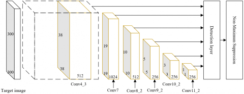
Figure 3. Structure of SSD network
Figure 3 shows the structure of SSD network. The multiscale feature map of SSD network is mainly extracted from the newly added convolutional layers. A total of six feature maps could be extracted, including Conv7, Conv8_2, Conv9_2, Conv10_2, Conv11_2, and Conv4_3. The sizes of the six feature maps are (38, 38), (19, 19), (10, 10), (5, 5), (3, 3), and (1, 1), respectively. The scale and aspect ratio of the priori box were configured based on the linear increasing rule. The number of priori boxes in each unit varies with the feature maps.
With each point on the feature map as the center, concentric default boxes of different scales were generated. With the growing number of pooling layers, the visible range of the feature map gradually increased, while the map size gradually decreased. However, the scale Ol of the default box increased linearly. Let Omin, and Omaxbe the scales of the bottom layer and the top layer, respectively. Then, Ol can be calculated by:
${{O}_{l}}={{O}_{min}}+\frac{{{O}_{max}}-{{O}_{min}}}{n-1}\left( l-1 \right),l\in \left[ 1,n \right]$ (13)
The six default boxes of various sizes can be obtained by the above formula (13). The default aspect ratio βS of the default boxes can be described as:
${{\beta }_{S}}\in \left\{ 1,2,3,\frac{1}{2},\frac{1}{3} \right\}$ (14)
Let EB and TA be the effective width and actual height of each default box, respectively. We have:
$\left\{ \begin{matrix} EB_{l}^{\beta }={{O}_{l}}\sqrt{{{\beta }_{S}}} \\ TA_{l}^{\beta }=\frac{{{O}_{l}}}{\sqrt{{{\beta }_{S}}}} \\ \end{matrix} \right.$ (15)
For the EfficientNet algorithm with spatial attention mechanism, the SSD network has the following convolutional layers: Conv7, Conv15, Conv22, Conv23_2, Conv24_2, and Conv25_2, whose sizes are (28, 28), (14, 14), (7, 7), (5, 5), (3, 3), and (1, 1), respectively. Based on focal loss function, the improved SSD network applies to the mining of difficult samples with weak metal surface defects.
During the design of network loss function, two convolutional layers with kernel size of 3×3 were introduced in turn to compute the output of a specific convolutional layer in the network. The loss function of the network is the weighted sum of confidence error and position error. Let MPS be the number of positive samples in the matched default box; d be the predicted class confidence; k be the predicted boundary coordinates of the default box; p be the location parameter of the actual box; LossRE and LossPO be the confidence error and position error of metal surface defects, respectively; γ be the weight coefficient obtained through cross validation. Then, the loss function can be obtained by:
$\begin{align} & Loss\left( a,d,k,p \right) \\ & =\frac{1}{{{M}_{PS}}}\left( Los{{s}_{RE}}\left( a,d \right)+\gamma Los{{s}_{PO}}\left( a,k,p \right) \right) \\ \end{align}$ (16)
where, the confidence error LossRE is generally calculated based on softmax error:
$Los{{s}_{RE}}\left( a,d \right)=-\sum\limits_{i\in Pos\text{ }}^{M}{a_{ij}^{t}log\left( \hat{d}_{i}^{t} \right)-}\sum\limits_{i\in Neg}{log\left( \hat{d}_{i}^{0} \right)}$ (17)
where,
$\hat{d}_{i}^{t}=\frac{{{e}^{d_{i}^{t}}}}{\sum\limits_{t}{{{e}^{d_{i}^{t}}}}}$ (18)
atij is a binary function; if atij=1, default box i matches with the ground truth box j in sample class t; if atij=0, the two boxes do not match with each other.
The position error LossPO is calculated by Smooth L1 loss:
$Los{{s}_{PO}}\left( a,k,p \right)=\sum\limits_{i\in Pos\text{ }}^{M}{\sum\limits_{n\in \left\{ da,db,EB,TA \right\}}{a_{ij}^{l}S{{L}_{L1}}\left( k_{i}^{n}-\hat{p}_{j}^{n} \right)}}$ (19)
$\left\{ \begin{matrix} \hat{p}_{j}^{da}=\left( p_{j}^{da}-v_{i}^{da} \right)/v_{i}^{EB} \\ \hat{p}_{j}^{db}=\left( p_{j}^{db}-v_{i}^{db} \right)/v_{i}^{TA} \\ \hat{p}_{j}^{EB}=log\left( {p_{j}^{EB}}/{v_{i}^{EB}}\; \right) \\ \hat{p}_{j}^{TA}=log\left( {p_{j}^{TA}}/{v_{i}^{TA}}\; \right) \\ \end{matrix} \right.$ (20)
alij is also a binary function; if alij=1, default box i matches with the ground truth box j in sample class 1; if atij=0, the two boxes do not match with each other. Suppose the predicted boundary coordinates k of the default box is the coded value. The position parameter p of the ground truth box needs to be encoded to obtain the parameter values of formula (20).
Let e be the difference between ground truth box and predicted box. Then, Smooth L1 loss function SLL1(a) can be given by:
$S{{L}_{{{L}_{1}}}}\left( e \right)=\left\{ \begin{align} & 0.5{{e}^{2}}\text{ }if\left| e \right|<1 \\ & \left| e \right|-0.5\text{ }otherwise \\ \end{align} \right.$ (21)
During metal surface image processing, the input target image is mostly the background of metal surface, that is, the defect area occupies a very small portion in the target image. If the background is overfitted, it would be very likely for the network fail to converge. Focal loss can effectively overcome the serious imbalance between positive and negative samples in target detection, such that the neural network will not over-predict the background samples, but focus on the learning of difficult samples with weak surface defects. Let b be the result of activation function, which falls in [0, 1]. Then, the focal loss can be calculated by:
$FL=-blog\left( b' \right)-\left( 1-b \right)log\left( 1-b' \right)$ (22)
When there is a huge amount of image data, the loss function will consume a long time in continuous calculation. This paper modifies the focal loss function with binary cross entropy:
$GD\left( {{t}_{\tau }} \right)={{\kappa }_{\tau }}{{\left( 1-{{\eta }_{\tau }} \right)}^{\upsilon }}log\left( {{\eta }_{\tau }} \right)$ (23)
Let ητ be the probability of detecting images with differences; υ be a constant falling in (0, +ꝏ); κτ be the adjustment factor for the proportion of positive samples to negative samples in all samples; κτand 1-κτ be the class of foreground and the class of background, respectively. Both κτ and 1-κτ are probabilities within [0, 1]. The above analysis shows that υ and κτ are constants, that need not to be trained during network training.
4.2 Feature fusion
The SSD network lacks information interaction between low- and high-level features. Drawing on the idea of feature pyramid network (FPN), this paper reconstructs a neural network that fuses high- and low-level features. The backbone network can simultaneously extract high-level semantics, and fuse the features of some high-level information and low-level information.
The traditional feature layer fusion mainly involves two operations: concatenate and add. The former combines the channels of multiple feature maps of the same size, while the latter superimposes the feature information of the pixels on the feature maps of the same size. Based on concatenate operation, add operation shares convolution kernels, reduces the computing load in the case of feature maps with wide channels, and effectively improves detection speed. This paper chooses add operation to fuse the metal surface defect features:
$W{{S}_{ADD}}=\sum\limits_{i=1}^{h}{{{u}_{i}}\left( {{A}_{i}}+{{B}_{i}} \right)}=\sum\limits_{i=1}^{h}{{{A}_{i}}}{{u}_{i}}+\sum\limits_{i=1}^{h}{{{B}_{i}}}{{u}_{i}}$ (24)
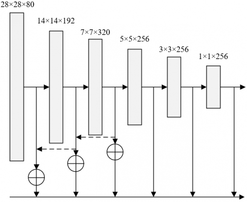
Figure 4. Structure of improved SSD feature fusion network
During neural network reconstruction, the feature fusion of Conv10_2, and Conv11_2 does not improve the detection effect. In actual practice, the two features may not be fused. Figure 4 shows the structure of the improved SSD feature fusion network. It can be inferred that, the add operation can integrate the different backbone networks of SSD with FPN. The integration will not increase the dimension of feature map, but embed richer information to the feature map on the lower level. In this way, the recognition performance will be improved for metal surface defects.
This paper evaluates defect detection effect with accuracy, precision, and recall. Let TP and TP be the number of correctly and incorrectly detected metal surface defects of the same type, respectively; TN be the number of correctly detected and judged metal surface defects of other types; FN be the number of failures in detecting any metal surface defect of any type. Then, the accuracy AC, which reflects whether the correct result is detected, can be calculated by:
$AC=\frac{TP+TN}{TP+TN+FP+FN}$ (25)
The precision, PR, which judges whether the detection result is an actual defect, can be calculated by:
$PR=\frac{TP}{TP+FP}$ (26)
The recall, RE, which judges whether the positive samples in the original image are detected as positive samples:
$recall=\frac{TP}{TP+FN}$ (27)
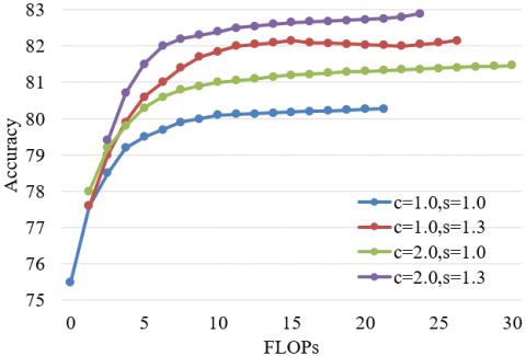
Figure 5. Accuracies of defect detection with different width coefficients
The same depth coefficient was configured for the neural network. Figure 5 shows the detection accuracies of different types of metal surface defects by EfficientNet scaled with different width coefficients. It can be learned that, if network depth coefficient u and image resolution coefficient s are fixed, and only width coefficient c is adjusted, the network accuracy of defect detection will soon saturate. If the depth coefficient u is fixed, while resolution coefficient s and width coefficient c are adjusted, the defect detection would be more accurate than that under single-dimensional scaling with the same computing cost. To sum up, the three dimensions should not be blindly expanded. Instead, the scales of different dimensions should be weighed carefully, such as to realize an ideal detection accuracy and the best network efficiency.
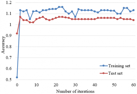
The EfficientNet with spatial attention mechanism was adopted for network training, in the light of the size of metal surface image, and the limitation of computing resources. To compare the EfficientNet qualities before and after the addition of spatial attention, this paper configures the same parameters values for the contrastive networks. Under the premise of ensuring model efficiency and detection accuracy, the authors analyzed only how the addition of spatial attention influences the network. Every other model parameter was obtained in reference to accuracy and loss function. If the two reference metrics are stable at the same time, the selected model has the optimal number of iterations. Figures 6 and 7 show the accuracy and loss curves of network models on training set and test set, respectively. It can be observed that, after 30 iterations, the accuracy and loss of the EfficientNet coupled with spatial attention tended to be stable. Further comparison shows the addition of spatial attention pushed up the network detection accuracy, and reduced the loss function.
Figure 6. Accuracy curve of EfficientNet with spatial attention mechanism
Figure 7. Loss curve of EfficientNet with spatial attention mechanism
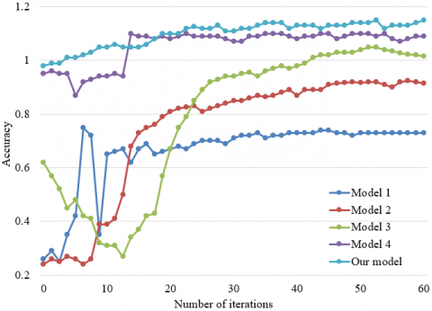
Next, the accuracy of the proposed network was compared with that of common defect classification and recognition models, aiming to demonstrate the effectiveness of EfficientNet more intuitively with attention mechanism in detecting different types of metal surface defects. The contrastive models include 1-VGG16, 2-ResNet50, 3-MobileNetV2, and 4-traditional EfficientNet. Figure 8 compares the detection accuracies of different models. Table 2 presents the detection accuracies, theoretical computing loads, and parameter quantities of different models. It can be seen that the addition of spatial attention mechanism to EfficientNet not only enhanced the key features of the defects of different types in the target image, but also ensured the information exchange between feature maps on different levels, thereby achieving better detection effect on metal surface defect image set.
Figure 8. Detection accuracies of different models
Table 2. Comparison of experimental results
|
Model |
Theoretical computing load FLOPS |
Parameter quantity |
Detection accuracy |
|
Model 1 |
267.4M |
135.7M |
72.56 |
|
Model 2 |
48.9M |
24.7M |
92.79 |
|
Model 3 |
4.8M |
2.5M |
89.20 |
|
Model 4 |
13.5M |
6.7M |
97.67 |
|
Our model |
13.5M |
6.7M |
98.21 |
Next is to verify the effectiveness of adopting improved SSD network to detect different types of metal surface defects. For this purpose, the non-maximum suppression layer, a key layer in the network, was verified first. Figure 9 shows the detection process of different types of metal surface defects: Initially, lots of default boxes are obtained, and the positive defect samples in the target image are marked in red boxes; Next, network detection, regression, and top-k selection are performed to effectively reduce the boxes for positive samples of defects; Finally, non-maximum suppression is carried out to re-filter the default boxes, and obtain the detection results on defects. The iterative execution of non-maximization suppression can optimize some bounding boxes that are partially repetitive, incorrect, or inaccurate.
Table 3 compares the experimental results of FPNs with different backbone networks. The contrastive neural networks include VGG16, VGG16 coupled with FPN, and improved SSD. It can be observed that the two backbone networks improved VGG16 and improved SSD achieved better detection time per target image and mean detection precision than VGG16 and SSD, thanks to the improvement of FPN coupling. In particular, the SSD improved by FPN in this paper reached the mean detection precision of 90%, and a single-image detection speed of 41.8ms, on metal surface defect image set. The performance could satisfy the ideal detection needs. The original SSD, which is not improved by FPN, was 5% smaller in mean detection precision, and 4.9 ms longer in detection speed, than our network. The results confirm the superiority of our algorithm.
Table 3. Experimental results of FPNs with different backbone networks
|
Model structure |
Mean precision |
Detection time |
|
VGG16 |
62% |
128.6 |
|
Improved VGG16 |
68% |
127.9 |
|
SSD |
85% |
46.7 |
|
Improved SSD |
90% |
41.8 |
Figure 9. Detection process of different types of metal surface defects
This paper explores the detection of various types of metal surface defects based on image processing. Firstly, the preprocessing method was given for metal surface images. Next, the EfficientNet was improved by adding the spatial attention mechanism for metal surface defect classification. After that, the backbone network of SSD was improved to realize feature fusion of the target image. Through experiments, the same depth coefficient was set for neural networks, and the detection accuracies of different types of metal surface defects were recorded for EfficientNet scaled with different width coefficients. The experimental results demonstrate that the scales of different dimensions should be weighed carefully, such as to realize an ideal detection accuracy and the best network efficiency. Furthermore, the accuracy and loss curves of network models on training set and test set were plotted, and a comparative experiment was conducted to verify that the network with attention mechanism achieved better detection accuracy than the original mechanism. Finally, the superiority of our algorithm was verified through comparison between FPNs with different backbone networks.
The study was supported by Jilin Province science and technology development, China (Grant No.: 20180201129GX).
[1] Bose, D., Guha, A. (2021). Economic production lot sizing under imperfect quality, on-line inspection, and inspection errors: Full vs. sampling inspection. Computers & Industrial Engineering, 160: 107565. https://doi.org/10.1016/j.cie.2021.107565
[2] Kardovskyi, Y., Moon, S. (2021). Artificial intelligence quality inspection of steel bars installation by integrating mask R-CNN and stereo vision. Automation in Construction, 130: 103850. https://doi.org/10.1016/j.autcon.2021.103850
[3] Leger, A., Le Goic, G., Fauvet, É., Fofi, D., Kornalewski, R. (2021). R-CNN based automated visual inspection system for engine parts quality assessment. In Fifteenth International Conference on Quality Control by Artificial Vision, 11794: 1179412. https://doi.org/10.1117/12.2586575
[4] Moru, D.K., Borro, D. (2020). A machine vision algorithm for quality control inspection of gears. The International Journal of Advanced Manufacturing Technology, 106(1): 105-123. https://doi.org/10.1007/s00170-019-04426-2
[5] Liu, Z., Qu, B. (2021). Machine vision based online detection of PCB defect. Microprocessors and Microsystems, 82: 103807. https://doi.org/10.1016/j.micpro.2020.103807
[6] Su, C., Hu, J.L., Hua, D., Cui, P.Y., Ji, G.Y. (2020). Micro image surface defect detection technology based on machine vision big data analysis. International Conference on Advanced Hybrid Information Processing, Binzhou, China, pp. 433-441. https://doi.org/10.1007/978-3-030-67874-6_40
[7] Kumar, R.P., Deivanathan, R., Jegadeeshwaran, R. (2020). Welding defect identification with machine vision system using machine learning. Journal of Physics: Conference Series, 1716(1): 012023. https://doi.org/10.1088/1742-6596/1716/1/012023
[8] Xue, B., Wu, Z. (2021). Key technologies of steel plate surface defect detection system based on artificial intelligence machine vision. Wireless Communications and Mobile Computing. https://doi.org/10.1155/2021/5553470
[9] Eshkevari, M., Rezaee, M.J., Zarinbal, M., Izadbakhsh, H. (2021). Automatic dimensional defect detection for glass vials based on machine vision: a heuristic segmentation method. Journal of Manufacturing Processes, 68: 973-989. https://doi.org/10.1016/j.jmapro.2021.06.018
[10] Zhou, Q., Chen, R., Huang, B., Liu, C., Yu, J., Yu, X. (2019). An automatic surface defect inspection system for automobiles using machine vision methods. Sensors, 19(3): 644. https://doi.org/10.3390/s19030644
[11] Ai, Y., Zhang, Y., Cao, X., Zhang, W. (2021). A defect detection method for the surface of metal materials based on an adaptive ultrasound pulse excitation device and infrared thermal imaging technology. Complexity. https://doi.org/10.1155/2021/8199013
[12] Lin, H.I., Wibowo, F.S. (2021). Image Data Assessment Approach for Deep Learning-Based Metal Surface Defect-Detection Systems. IEEE Access, 9: 47621-47638. https://doi.org/10.1109/ACCESS.2021.3068256
[13] Feng, W., Liu, H., Zhao, D., Xu, X. (2020). Research on defect detection method for high-reflective-metal surface based on high dynamic range imaging. Optik, 206: 164349. https://doi.org/10.1016/j.ijleo.2020.164349
[14] Di Cataldo, S., Vinco, S., Urgese,., Calignano, F., Ficarra, E., Macii, A., Macii, E. (2021). Optimizing quality inspection and control in powder bed metal additive manufacturing: Challenges and research directions. Proceedings of the IEEE, 109(4): 326-346. https://doi.org/10.1109/JPROC.2021.3054628
[15] Sun, H., Liu, Z., Zhang, J. (2021). Defect-sensitive testing data analysis method for industrial robots quality inspection. In 2021 IEEE 10th Data Driven Control and Learning Systems Conference (DDCLS), Suzhou, China, pp. 513-517. https://doi.org/10.1109/DDCLS52934.2021.9455637
[16] Gutierrez, P., Luschkova, M., Cordier, A., Shukor, M., Schappert, M., Dahmen, T. (2021). Synthetic training data generation for deep learning based quality inspection. arXiv preprint arXiv:2104.02980.
[17] Liu, Z., Tang, R., Duan, G., Tan, J. (2021). TruingDet: Towards high-quality visual automatic defect inspection for mental surface. Optics and Lasers in Engineering, 138: 106423. https://doi.org/10.1016/j.optlaseng.2020.106423
[18] Lin, H.I., Lin, P.Y. (2020). An image quality assessment method for surface defect inspection. 2020 IEEE International Conference on Artificial Intelligence Testing (AITest), Oxford, UK, pp. 1-6. https://doi.org/10.1109/AITEST49225.2020.00008
[19] Hu, J., Yan, P., Su, Y., Wu, D., Zhou, H. (2021). A Method for Classification of Surface Defect on Metal Workpieces based on Twin Attention Mechanism Generative Adversarial Network. IEEE Sensors Journal, 21(12): 13430-13441. https://doi.org/10.1109/JSEN.2021.3066603
[20] Zhou, A., Zheng, H., Li, M., Shao, W. (2020). Defect inspection algorithm of metal surface based on machine vision. 2020 12th International Conference on Measuring Technology and Mechatronics Automation (ICMTMA), Phuket, Thailand, pp. 45-49. https://doi.org/10.1109/ICMTMA50254.2020.00017