Makbule Hilal Mütevelli* | Semih Ergin
© 2021 IIETA. This article is published by IIETA and is licensed under the CC BY 4.0 license (http://creativecommons.org/licenses/by/4.0/).
OPEN ACCESS
Accurate and automatic detections of brain tumors are vital. The aim of this study is to detect brain tumors in Magnetic Resonance (MR) images and to classify these tumors with a high degree of accuracy. After removing skull, the suspicious regions including tumors in the MR images were detected by using K-means clustering, K-means clustering in Lab color space, and the Chan-Vese without edges algorithm. At this stage, a performance evaluation of these three different methods was investigated, and it was seen that the best result was obtained in the Chan-Vese active contour without edges algorithm. For the classification stage, various features such as shape-based features, gray level co-occurrence matrix features, histogram of oriented gradients features, local binary pattern features, and statistical features were extracted from the detected suspicious regions. Finally, the suspicious regions were classified by k-nearest neighbor (k-NN), Fisher’s linear discriminant analysis (FLDA), random forest, decision tree, support vector machines (SVM), logistic linear classifier (LLC), and Naive Bayes classification methods. As a result of this study, it was determined that the FLDA classifier provided the best results with 93.01% accuracy, 93.46% sensitivity, and 96.50% specificity rates in classification for benign tumors, malignant tumors, and healthy (without tumor) cases.
brain tumor, computer aided detection, skull removal, suspicious region detection
Tumors consist of brain cells, glands, and nerves around the cerebral cortex. A brain tumor occurs due to the abnormal growth of cells. Brain tumors can directly destroy brain cells, and they can damage the cells by applying pressure to the skull [1]. A benign tumor grows slowly. Even if it is not cancerous, it can cause serious problems by putting pressure on some parts of the brain when it reaches a certain size. In rare cases, it can turn into a malignant tumor over time. A malignant tumor grows very quickly; it extends into the healthy structures around it and seriously damages these structures. It consists of cells that grow uncontrollably and is often referred to as cancer [2]. Brain tumor is one of the brain diseases that cause death the most frequently; therefore, early diagnosis of brain tumor is very important. The most commonly used imaging technique in the detection of brain tumors is magnetic resonance imaging (MRI). MRI scans the organs and soft tissues in the body in detail using a strong magnetic field and radio waves, and it is more useful because it does not use radiation [3].
Today, the detection of tumors is done by radiologists and doctors via MRI. However, this method is not always fast and accurate. For this reason, Computer Aided Detection (CAD) systems have been developed to minimize the errors caused by imaging techniques and radiologists [4].
The similarity of the density of skull and brain tissue in MRI images makes difficult tumor detection; therefore, the skull needs to be removed from MRI images, and there are many studies on this subject [5, 6]. Arakeri and Reddy stated that removing the skull from the MRI image is an important step in segmentation, and they converted the original T2-weighted MRI image to a binary image using a threshold value calculated automatically using Otsu’s method. The resulting image consists of connected components. Then, they searched for the largest connected component corresponding to the brain and eliminated the skull region by holding only the pixels in the largest connected component [7]. Anitha and Murugavalli extracted the brain region from the skull using the skull stripping technique after completing the de-noising process for MRI images [8]. They first converted the original MR images to a binary image using a low threshold value via Otsu’s method. Finally, the authors applied mathematical morphology operations including erosion, dilation, and region filling to the resultant image.
Suspicious region detection is an important segmentation process for an accurate classification stage, and various methods are used for detection. Sehgal et al. [1] proposed a fully automatic method to detect brain tumors in MRI images. They segmented the images using the fuzzy C-means technique. For tumor extraction, the authors used area and circularity as criteria. Finally, they verified the results by comparing with the manually segmented ground truth. Amin et al. presented an automated system for detecting brain tumor at lesion and image levels in MRI [3]. At the image level, they used the Gaussian filter for image smoothing and applied the optimal threshold value and various morphological operations. At the lesion level, they converted the input image to Lab color space. Then, the authors applied the K-means clustering method and some morphological operations. Mandwe and Anjum proposed a computer aided system for brain MRI image segmentation. In this system, they used clustering techniques such as K-means clustering and fuzzy C-means clustering [9]. Zawish et al. suggested an advanced image segmentation technique based on variation methods to accurately segment tumors from the brain MRI. This technique is based on the Chan-Vese active contour without edges algorithm. They tested and verified the effectiveness of the algorithm on different brain MRI images [10].
The choice of classifiers is very important in classification problems, and here are many studies on classification in the literature. Sachdeva et al. used principal component analysis (PCA) to reduce the feature space dimension and artificial neural network (ANN) for classification [11]. They first classified feature vectors using ANN and subsequently classified them using the PCA-ANN approach. It was seen that the classification accuracy rate increased from 77 to 91%. Praveen and Agrawal presented hybrid approach for brain tumor classification. They classified normal and abnormal MRI images using the least squares SVM classifier with a classification accuracy of 96.63% [12]. Wasule and Sonar classified extracted GLCM features using the SVM and k-NN methods. The accuracy rate achieved was 96% and 86% for SVM and KNN, respectively, for the clinical database [13]. Asodekar and Gore extracted shape-based features for the classification of benign and malignant tumors. Then, they classified them using random forest with an accuracy of 81.90% and SVM with an accuracy of 78.57% [14].
In this study, an automatic system that detects brain tumors in MRI images and classifies these tumors was presented. This system consisted of four phases, skull removal, suspicious region detection, feature extraction and classification. The skull was removed by utilizing binarization method and morphological operations. Different algorithms such as K-means clustering, K-means clustering in Lab color space and Chan-Vese active contour without edges were applied to detect suspicious regions, and it was seen that the Chan-Vese active contour without edges algorithm gives the best performance for the detection of suspicious regions. Then intensity, texture, and shape-based features were extracted from suspicious regions detected in the MRI images. Seven different classifiers were applied for classification. Finally, the suspicious regions were classified into three classes, benign tumor, malignant tumor, and normal.
Removing of the skull is an important step in the detection of a brain tumor in MR images [6]. The similarity in density of the skull and brain tissue in the MR images of the brain makes it difficult to detect suspicious regions. For this reason, the skull is removed to accurately determine the tumor region. In this study, the binarization method, different morphological operations and image masking were used to remove the skull. Image binarization is a method used as a preprocessor that converts grayscale image to a binary image (black or white) at a certain threshold value [15].
3.1 K-means clustering
Clustering methods group objects according to some qualities and characteristics. K-means clustering is one of the most commonly used clustering methods to segment an image.
K-means clustering aims to segment images into K clusters by minimizing error of square [16]. In the K-means algorithm, the number of clusters K is initially defined. Then, K centers are selected randomly for each cluster. The distance between each data point and each cluster center is calculated by using Euclidean measurement method. The distances of a single data point to each cluster center are compared with each other, and this data point is assigned to a cluster whose distance is minimum among all clusters. The center of each cluster is then recomputed. The distances are recalculated and compared with each other again. The process is continued until the data point is not assigned to the cluster [17]. The new centers of the clusters are determined by calculating the averages.
In the K-means clustering algorithm, the distance between the data and the cluster centers is calculated as shown in Eq. (1). The error sum of squares (SSE) is the Euclidean distance of the data points to x center. ci denotes ith center, and K denotes the number of cluster centers.
$S S E=\sum_{i=1}^{K} \sum_{x \in c_{i}} \operatorname{dist}^{2}\left(c_{i}, x\right)$ (1)
3.2 K-means clustering in Lab color space
Color space is identified as a set of possible colors in a particular color organization. In general, three basic colors (red, green, blue) are used. A variety of colors is provided when these basic colors are changed at different rates [18].
Lab color space is one of the color spaces that have separate brightness and color channels. Components of the Lab color space are denoted as L (lightness), a (red/green axis) and b (yellow/blue axis). This color space has three coordinates. The L value represents the lightness or brightness of the color in the image, and the value of L ranges from 0 (black) to 100 (white). As L value increases, the colors become brighter. a and b values range from -128 to +127. a represents the amount of green (−) or red (+) components in the image. b represents the amount of blue (−) or yellow (+) components in the image [19].
In K-mean clustering in Lab color space, input image is converted to the Lab color space. Input RGB-colored image is first converted to XYZ color space; then, XYZ color space is converted to Lab color space with Eq. (2) and Eq. (3). In Eq. (3), f is a function which defines L, a and b components. In this paper, the Illuminant D65 Standard is used and $X_{n}$, $Y_{n}$, $Z_{n}$ are selected as 95.0489, 100, 108.8840, respectively.
$L=116 f\left(\frac{Y}{Y_{n}}\right)-16$
$a=500\left[f\left(\frac{X}{X_{n}}\right)-f\left(\frac{Y}{Y_{n}}\right)\right]$
$b=200\left[f\left(\frac{Y}{Y_{n}}\right)-f\left(\frac{Z}{Z_{n}}\right)\right]$ (2)
$t=\frac{X}{X_{n}}, \frac{Y}{Y_{n}} \operatorname{or} \frac{Z}{Z_{n}}, \quad \delta=\frac{6}{29}$
$f(t)=\left\{\begin{array}{r}\sqrt[3]{t} \text { if } t>\delta^{3} \\ \frac{t}{3 \delta^{2}}+\frac{4}{29} \text { otherwise }\end{array}\right.$ (3)
Then, the image is segmented by applying the K-means clustering algorithm. Lab color space is preferred in many image analyses because it is a color space with a perceptually uniform distribution [3, 18].
3.3 Chan-Vese active contour model without edges
The Chan-Vese active contour model without edges is a region-based segmentation method. This model uses curve (contour) evolution and level set method. It does not depend on the gradient of the image to end the contour evolution on the boundaries of the region of interest [20]. The Chan-Vese algorithm is based on the Mumford-Shah model that uses energy function for image segmentation [21].
In the Chan-Vese active contour algorithm, the energy function formularized for the intensity of the u0 image in the point (x, y) separated by C contour into two regions is given in Eq. (4) [20].
$F\left(c_{1}, c_{2}, C\right)$
$=\mu .$ Length $(C)$
$+v .$ Area $($ inside $(C))+\lambda_{1} \int_{i n s i d e(C)} \mid u_{0}(x, y)$
$-\left.c_{1}\right|^{2} d x d y+\lambda_{2} \int_{\text {outside( } C)}\left|u_{0}(x, y)-c_{2}\right|^{2} d x d y$ (4)
In the equation, $\mu \geq 0, v \geq 0, \lambda_{1}, \lambda_{2}>0$ are fixed parameters. Chan and Vese fix $\lambda_{1}=\lambda_{2}=1$ and $v=0$ in their algorithms. Thus, the energy function is minimized as shown in Eq. (5). $c_{1}$ is the average intensity value of the region inside the C contour, and $c_{2}$ is the average intensity value of the region outside the C contour. $F_{1}(C)$ and $F_{2}(C)$ are defined as force terms.
$\begin{aligned} F_{\min }\left(c_{1}, c_{2}, C\right)=& \mu . \operatorname{Length}(C) \\ &+\int_{i n side(C)}\left|u_{0}(x, y)-c_{1}\right|^{2} d x d y \\ &+\int_{{outside}(C)}\left|u_{0}(x, y)-c_{2}\right|^{2} d x d y \\ &=\mu . \operatorname{Length}(C)+F_{1}(C)+F_{2}(C) \end{aligned}$ (5)
In the Chan-Vese model without edges, ϕ(x,y) is the level set function that shows contour values. The mathematical notation of the C contour is shown in Eq. (6), and the change of this contour over time according to the ϕ(x,y) function is shown in Eq. (7).
$C=\{(x, y): \phi(x, y)=0\}, \forall(x, y) \in u_{0}$ (6)
$\frac{\partial C}{\partial t}=\frac{\partial \phi(x, y)}{\partial t}$ (7)
In the $F\left(c_{1}, c_{2}, C\right)$ energy function, the $F_{1}(C)$ force term shrinks the contour while the $F_{2}(C)$ force term expands the contour. When the contour reaches the boundary of the regions of interest, these two forces are balanced, thus allowing the contour of the region to be found. The operating logic of the Chan-Vese algorithm is illustrated in Figure 1. In the figure, black places indicating the region of interest are denoted with a value of -1 and gray places indicating places outside the region of interest are denoted with a value of +1. A white curve represents the contour. In case 1, the contour covers the whole region of interest (-1) and some gray places (+1). Thus, $c_{1} \cong 0$ and $c_{2}=1$. According to the $F\left(c_{1}, c_{2}, C\right)$ energy function, $F_{1}>0$ and $F_{2} \approx 0$ are obtained. Therefore, the algorithm shrinks the contour. Similar operations occur in other cases. Finally, when the contour reaches the boundary of the region, as in case 4, $F_{1} \approx 0$ and $F_{2} \approx 0$, the forces are balanced and contour of the region is found.
Figure 1. The operating logic of the Chan-Vese algorithm [20]
4.1 Shape-based features
Brain tumors can vary greatly in terms of size, the diversity of their borders, and regularity or irregularity [22]. Shape-based features have a distinctive property in the analysis of these brain tumors. The largest interconnected object is found in a detected suspicious region. For each the largest interconnected object in a binary image, eleven different shape-based features are extracted. These features are described below.
The perimeter is the total number of pixels on the boundary of the object. The area is the total number of pixels in the object. The convex area is the total number of pixels in the smallest convex containing the object. The solidity is computed by the ratio of area to convex area. The fullness ratio is found by the ratio of the total number of pixels (area) in the object to the total number of pixels in the smallest rectangle containing the object. The major axis length is the number of pixels in the longest diameter of the ellipse containing the object. The minor axis length is the number of pixels in the shortest diameter of the ellipse containing the object. Eccentricity is found by the ratio of the distance between the focal points of the ellipse and the major axis length. Orientation is the angle between the major axis of the ellipse and x axis. The diameter (D) is computed by the diameter of a circle that has an area equal to the area of the object. It is found as in Eq. (8).
$D=\sqrt{\frac{4 * A r e a}{\Pi}}$ (8)
Roundness (Y) represents the degree of an object's similarity to a circular shape. It is found as in Eq. (9). r is the ratio of the major axis length to the minor axis length [23].
$Y=\frac{ { Area }}{\Pi r^{2}}$ (9)
4.2 Gray level co-occurrence matrix (GLCM) features
Second order statistical features extracted by using GLCM are defined as texture features [24]. GLCM indicates the spatial relationship between pixels with different gray levels.
The GLCM matrix is based on the function $P(i, j \mid d, \theta)$ which expresses the probability of gray levels at random distances and in whole image orientations. It is calculated by finding out how different a pixel with a specific intensity i is in relation to another pixel j in a specific distance d and orientation θ. Each element (i, j) in the GLCM matrix is the total number of times of occurrence of i and j pixel values according to one another in the specified relationship [25].
In the study, 22 different texture features suggested from the GLCM matrices calculated are extracted [24, 26-28]. Equations used for feature extraction are given in Table 1. $P(i, j)$ is the gray level co-occurrence matrix. $\mu_{x}$ and $\mu_{y}$ represent the average of the rows and columns of the GLCM respectively, and $\sigma_{x}$ and $\sigma_{y}$ represent the standard deviation of the rows and columns of the GLCM, respectively. The texture features and their mathematical representations are given in Table 2.
Table 1. Required equations
|
$P(i, j): G L C M=\left[\begin{array}{ccc}P(1,1) & \cdots & P\left(1, N_{g}\right) \\ \vdots & \ddots & \vdots \\ P\left(N_{g}, 1\right) & \cdots & P\left(N_{g}, N_{g}\right)\end{array}\right]$ |
|
$P_{x}(i)=\sum_{j=1}^{N_{g}} P(i, j), \quad P_{y}(i)=\sum_{i=1}^{N_{g}} P(i, j)$ |
|
$P_{x+y}(k)=\sum_{i=1}^{N_{g}} \sum_{j=1}^{N_{g}} P_{i+j=k}(i, j), k=2,3, \ldots, 2 N_{g}$ $P_{x-y}(k)=\sum_{i=1}^{N_{g}} \sum_{j=1}^{N_{g}} P_{|i-j|=k}(i, j), k=0,1, \ldots, N_{g}-1$ |
|
$\mu_{x}=\sum_{i} \sum_{j} i.P(i, j), \mu_{y}=\sum_{i} \sum_{j} j . P(i, j)$ |
|
$\sigma_{x}=\sum_{i} \sum_{j}\left(i-\mu_{x}\right)^{2} . P(i, j),$ $\sigma_{y}=\sum_{i} \sum_{j}\left(j-\mu_{y}\right)^{2} . P(i, j)$ |
4.3 Histogram of oriented gradients (HOG) features
HOG was first proposed for object detection purposes [29]. Then, it was also used for feature extraction purposes in computer vision and image processing [30].
Before the HOG features are extracted, an image is divided into cells. Then the edge direction and gradient values of the cells are evaluated. The main purpose here is to obtain local histograms of the image cells. The local histograms consist of gradient orientations. At first, the horizontal and vertical gradient values of the cells are calculated as in Eq. (10) and Eq. (11), respectively. Various edge detection masks are used in the x and y directions to calculate these values. $f_{x}(x, y)$ and $f_{y}(x, y)$ refers to the brightness change on the horizontal axis and the vertical axis, respectively.
$f_{x}(x, y)=I(x+1, y)-I(x-1, y)$ (10)
$f_{y}(x, y)=I(x, y+1)-I(x, y-1)$ (11)
Then, the magnitudes and orientations of the gradients are calculated by using the Eq. (12) and Eq. (13), respectively. m(x, y) represents the gradient magnitude, and θ(x, y) represents the gradient orientation. In this paper, the HOG features are extracted within the cells with the size of 9 x 9, and 9 different orientations are applied to these cells.
$m(x, y)=\sqrt{f_{x}(x, y)^{2}+f_{y}(x, y)^{2}}$ (12)
$\theta(x, y)=\tan ^{-1} \frac{f_{x}(x, y)}{f_{y}(x, y)}$ (13)
4.4 Local binary pattern (LBP) features
The basis of the LBP method is the texture analysis based on the texture units representing the local texture aspect in the image [31]. Texture features are obtained by using the LBP method. LBP creates a descriptor or texture model using the knowledge of the local texture neighbors surrounding each pixel [32].
The LBP operator generates a binary code by comparing each pixel with its neighbor pixels around it and creates a new pixel value. Each center pixel is compared with a certain number of neighbors in its neighborhood. If the neighbor pixel is greater than or equal to the center pixel, it has a value of 1, but if the neighbor pixel is smaller than the center pixel, it has a value of 0. The decimal value of the binary code created with these values becomes the new value of the center pixel.
The mathematical representation of LBP is given in Eq. (14). In the equation, P represents the number of pixels in a circular neighborhood, and R represents the radius of the circle. s is the unit step function. $g_{p}(p=0, \ldots, P-1)$ and $g_{c}$ denote the intensity value of the pth neighbour pixel in the circular neighborhood and the intensity value of the center pixel, respectively.
$x=g_{p}-g_{c}$
$s(x)=\left\{\begin{array}{l}1, x \geq 0 \\ 0, x<0\end{array}\right.$
$L B P(P, R)=\sum_{p=0}^{P-1} s\left(g_{p}-g_{c}\right) \cdot 2^{p}$ (14)
Table 2. GLCM texture features and their mathematical representations
|
GLCM texture features |
Mathematical representations |
|
Autocorrelation [26] |
$\sum_{i} \sum_{j}(i . j) . P(i, j)$ |
|
Contrast [24, 26] |
$\sum_{n=0}^{N_{g}-1} n^{2}\left\{\sum_{i=1}^{N_{g}} \sum_{j=1 \atop |i-j \mid=n}^{N_{g}} P(i, j)\right\}$ |
|
Correlation (MATLAB Suite) |
$\frac{\sum_{i} \sum_{j}\left(i-\mu_{x}\right) .\left(j-\mu_{y}\right) .(P(i, j))}{\sigma_{x} . \sigma_{y}}$ |
|
Correlation [24, 26] |
$\frac{\sum_{i} \sum_{j}(i . j) . P(i, j)-\mu_{x} . \mu_{y}}{\sigma_{x} . \sigma_{y}}$ |
|
Cluster Prominence [26] |
$\sum_{i=0}^{N_{g}-1} \sum_{j=0}^{N_{g}-1}\left\{i+j-\mu_{x}-\mu_{y}\right\}^{4} . P(i, j)$ |
|
Cluster Shade [26] |
$\sum_{i=0}^{N_{g}-1} \sum_{j=0}^{N_{g}-1}\left\{i+j-\mu_{x}-\mu_{y}\right\}^{3} . P(i, j)$ |
|
Dissimilarity [26] |
$\sum_{i} \sum_{j}|i-j| . P(i, j)$ |
|
Energy [24, 26] |
$\sum_{i} \sum_{j}\{P(i, j)\}^{2}$ |
|
Entropy [26] |
$-\sum_{i=0}^{N_{g}-1} \sum_{j=0}^{N_{g}-1} P(i, j) . \log \{P(i, j)\}$ |
|
Homogeneity (MATLAB Suite) |
$\sum_{i} \sum_{j} \frac{1}{1+|i-j|^{2}} . P(i, j)$ |
|
Homogeneity [26] |
$\sum_{i} \sum_{j} \frac{1}{1+(i-j)^{2}} . P(i, j)$ |
|
Maximum Probability [26] |
$\max _{i, j} P(i, j)$ |
|
Variance [24] |
$\sum_{i} \sum_{j}(i-\mu)^{2} . P(i, j)$ |
|
Sum Average [24] |
$\sum_{i=2}^{2 N_{g}} i . P_{x+y}(i)$ |
|
Sum Variance [24] |
$\sum_{i=2}^{2 N_{g}}(i-\text { Sum Average })^{2} . P_{x+y}(i)$ |
|
Sum Entropy [24] |
$-\sum_{i=2}^{2 N_{g}} P_{x+y}(i) . \log \left\{P_{x+y}(i)\right\}$ |
|
Difference Variance [24] |
variance of $P_{x-y}$ |
|
Difference Entropy [24] |
$-\sum_{i=2}^{2 N_{g}} P_{x-y}(i) . \log \left\{P_{x-y}(i)\right\}$ |
|
Information Measure of Correlation1 [24] |
$\frac{H X Y-H X Y 1}{\max \{H X ; H Y\}}$ $H X Y=-\sum_{i} \sum_{j} P(i, j) . \log (P(i, j))$ $H X Y 1=-\sum_{i} \sum_{j} P(i, j) . \log \left(p_{x}(i) . p_{y}(j)\right)$ HX and HY are entropies of $p_{x}$ and $p_{y}$ |
|
Information Measure of Correlation2 [24] |
$(1-\exp [-2 .(H X Y 2-H X Y)])^{1 / 2}$ $H X Y 2=-\sum_{i} \sum_{j} P_{x}(i) \cdot P_{y}(j) \cdot \log \left\{P_{x}(i) \cdot P_{y}(j)\right\}$ |
|
Inverse Difference Normalized [27] |
$\sum_{i}^{N_{g}} \sum_{j}^{N_{g}} \frac{1}{1+|i-j|^{2} / N_{g}^{2}} . P(i, j)$ |
|
Inverse Difference Moment Normalized [27] |
$\sum_{i}^{N_{g}} \sum_{j}^{N_{g}} \frac{1}{1+(i-j)^{2} / N_{g}{ }^{2}} . P(i, j)$ |
4.5 Statistical features
Statistical features are intensity-based features [33]. Statistical features used for an accurate classification are preferred in many studies. In this study, eight different statistical features were extracted from the suspicious regions detected in MR images. These features and their mathematical representations are given in Table 3.
Table 3. Statistical features and their mathematical representations
|
Statistical features |
Mathematical representations |
|
Energy |
$\sum_{i=1}^{N} x_{i}^{2}$ |
|
Mean |
$\mu=\frac{1}{N} \sum_{i=1}^{N} x_{i}$ |
|
Variance |
$\frac{1}{N-1} \sum_{i=1}^{N}\left(x_{i}-\mu\right)^{2}$ |
|
Skewness |
$\sigma=$ Standard Deviation $=\sqrt{\mu}$ $\frac{\frac{1}{N} \sum_{i=1}^{N}\left(x_{i}-\mu\right)^{3}}{\sigma^{3}}$ |
|
Kurtosis |
$\frac{\frac{1}{N} \sum_{i=1}^{N}\left(x_{i}-\mu\right)^{4}}{\sigma^{4}}$ |
|
Entropy |
$\sum_{i=1}^{N} p\left(x_{i}\right) \log _{2} p\left(x_{i}\right)$ |
|
Mean Energy |
$\mu_{\text {Energy }}=\frac{1}{N} \sum_{i=1}^{N} x_{i}^{2}$ |
|
Energy Variance |
$\frac{1}{N-1} \sum_{i=1}^{N}\left(x_{i}^{2}-\mu_{\text {Energy }}\right)^{2}$ |
5.1 Database
The Harvard database was used in the study [34]; it consists of 141 brain MR images, 41 of which are normal (healthy) and 100 of which contain tumors. Of the 100 images containing tumors, 59 of these are benign and 41 of these are malign. All the brain MR images used in the study have a 256 × 256-pixel size and an 8 bits depth.
5.2 Skull removal in MR images
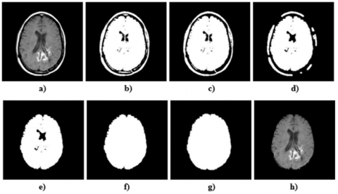
Skull removal in MR images is shown in Figure 2. Firstly, a random original input image in RGB format is converted to a grayscale image shown in Figure 2 a). Then, the binarization method is used [15]. The grayscale image is converted to a binary image using a selected the threshold value 55. The binary image is shown in Figure 2 b). The largest interconnected component in the binary image is obtained as seen in Figure 2 c). The skull and brain are connected to each other with small components. Opening, which is a morphological operation is applied to disconnect [35]. The resulting image is given in Figure 2 d). After the opening operation, the largest interconnected component is achieved again as shown in Figure 2 e). Thus, only the brain region is found. Then, the hole filling operation is applied to obtained the image, and the holes are filled as in Figure 2 f). To expand details and increase size, a dilation operation [36] is applied to the obtained image, as seen Figure 2 g). Thus, the necessary mask is found by stripping the skull. Finally, masking is performed to the grayscale image by using this mask and the skull is removed from the brain. The skull-stripped image is given in Figure 2 h).
Figure 2. Skull removal: a) grayscale image, b) binary image, c) the largest interconnected component, d) opening operation applied image, e) brain image, f) hole filling operation applied image, g) dilation operation applied image, h) skull-stripped image
5.3 Suspicious region detection in MR images
After the skull is removed, the suspicious region is detected in all MR images by using K-means clustering, K-means clustering in Lab color space, and the Chan-Vese active contour without edges algorithms.
Figure 3. Suspicious region detection with K-means clustering algorithm: a) a sample image, b) segmentation of suspicious region
Figure 4. Suspicious region detection with K-means clustering in Lab color space algorithm: a) image converted to Lab color space, b) segmentation of suspicious region
In the K-means clustering, each of the images in the training data is segmented using different number of clusters. Because of this reason, the mean of the number of clusters providing the best segmentation results is evaluated. The calculated value is approximately three. Therefore, the number of clusters is preferred as three. The K-means clustering algorithm is applied to a sample image given in Figure 3 a) and suspicious region detection is performed as in Figure 3. The white areas in Figure 3 b) indicate the suspicious region found by the algorithm.
In the K-means clustering in Lab color space, a sample image is converted to Lab color space, as shown in Figure 4 a). Then, the K-means clustering algorithm with three clusters is applied to the obtained image and the suspicious region detection is performed as in Figure 4. The red areas in Figure 4 b) indicate the suspicious region found by the algorithm.
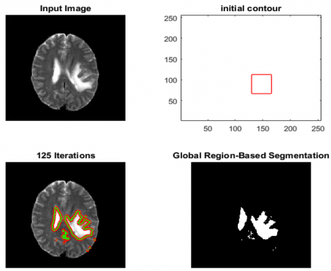
Figure 5. Suspicious region detection with Chan-Vese active contour without edges algorithm
In the Chan-Vese active contour without edges, the initial contour and number of iterations are determined. The Chan-Vese active contour without edges algorithm is applied to the input image, and suspicious region detection is performed as in Figure 5. The number of iterations is 125, and the weight of length term is selected as 0.9 in the Chan-Vese active contour without edges algorithm. The initial mask is a rectangular area and the x-coordinates of this area are between the pixels numbered as 145 and 190 whereas the y-coordinates of this area are between the pixels numbered as 130 and 165. Therefore, the size of mask is 46x36.
In the study, evaluation criteria given in Table 4 were used to measure the success in the suspicious region detection and classification stages.
Table 4. Performance evaluation criteria
|
TP: True Positive |
FP: False Positive |
|
FN: False Negative |
TN: True Negative |
|
Sensitivity - (SNS) = $\frac{T P}{(T P+F N)}$ Specificity - (SPC) = $\frac{T N}{(T N+F P)}$ Accuracy - (ACC) = $\frac{T P+T N}{(T P+T N+F P+F N)}$ |
|
Table 5. Confusion matrices and successes of algorithms
|
K-means clustering |
K-means clustering in Lab color space |
Chan-Vese active contour without edges |
|
TP=165281 FN=43848 FP=511107 TN=5833364 |
TP=148087 FN=61042 FP=391016 TN=5953455 |
TP=175131 FN=33998 FP=291571 TN=6052900 |
|
Sensitivity = 0.79 |
Sensitivity = 0.71 |
Sensitivity = 0.84 |
|
Specificity = 0.92 |
Specificity = 0.94 |
Specificity = 0.95 |
|
Accuracy = 0.92 |
Accuracy = 0.93 |
Accuracy = 0.95 |
A confusion matrix was found for each algorithm to measure the performance of the algorithms used. A performance evaluation of three different algorithms was made using these matrices. The confusion matrices and successes of the algorithms was given in Table 5. As a result, it is seen that the best result in the suspicious region detection belongs to the Chan-Vese active contour without edges algorithm.
5.4 Feature extraction on suspicious regions detected in MR images
Regions with the size of 64 x 64 were selected from the suspicious regions detected by three different algorithms, and feature extraction was obtained from these regions. All five different features (shape based, GLCM, HOG, LBP, statistical) were extracted separately, and feature vectors were created. The classification result of each feature vector was found. Then, the classification results of new feature vectors created in different combinations of the feature vectors obtained from suspicious regions determined by Chan-Vese active contour method were examined.
Shape-based features described in subsection 4 were extracted from the region 64 x 64 in size. The shape-based feature vector is created by using each of the three suspicious region detection algorithms and it is size 1 x 11. The GLCM matrix was calculated by taking $d=2$ and $\theta=0^{\circ}$ from the region of 64 x 64 in size. Then, the texture features given in Table 2 were extracted from the GLCM matrix. The GLCM feature vector is created by using each three suspicious region detection algorithms and it is 1 x 22 in size. The HOG feature vector is created by using K-means clustering and K-means clustering in Lab color space algorithms and it is 1 x 3136 in size. The HOG features were extracted within the cells with the size of 8 x 8, and 16 different orientations were applied to these cells. The HOG feature vector is also created by using the Chan-Vese active contour algorithm and it is 1 x 1216 in size. The HOG features were extracted within the cells with the size of 9 x 9, and 9 different orientations were applied to these cells. The LBP feature vector is created by using each three suspicious region detection algorithms and it is 1 x 944 in size. The LBP features were extracted from a region with the size of 64 x 64 obtained by using the K-means clustering algorithm. The radius of the circle is 2, and the number of neighbors is 8. The LBP features were extracted from a region with the size of 64x64 obtained by using K-means clustering in Lab color space and Chan-Vese active contour algorithms. The radius of the circle is 5, and number of neighbors is 8. To extract the statistical features, a matrix with the size of 64 x 64 was converted into a vector with the size of 1 x 4096. Energy, mean, variance, skewness, kurtosis, entropy, average energy, and energy variance features were extracted from a region with the size of 1 x 4096 obtained by using the K-means clustering algorithm. The created feature vector is 1 x 8 in size. Energy, mean, variance, skewness, kurtosis, and entropy features were extracted from a region with the size of 1 x 4096 obtained by using K-means clustering in Lab color space and Chan-Vese active contour algorithms. The created feature vector is 1 x 6 in size.
5.5 Classification of suspicious regions
The suspicious regions were classified by k-NN (k = 1) [37], FLDA [38], random forest (number of trees = 100) [39], decision tree [40], SVM [41], LLC [42, 43], and Naive Bayes [44] classifiers. This classification has three classes (benign tumor, malignant tumor, and normal). 66% of each class was chosen as training data and 34% as test data. A 3-fold cross-validation technique was used for classification. This technique has three stages, and, for each stage, a different 34% of the classes were used as test data. Accuracy, sensitivity, and specificity rates were obtained for each stage to calculate the classification result. These obtained values were summed and averaged so that general classification result was calculated.
The classification results of five different feature vectors created by using K-means clustering algorithm were calculated separately. For each classifier, the classification results calculated by using 11-dimensional shape-based features, the classification results calculated by using 22-dimensional GLCM features, the classification results calculated by using 3136-dimensional HOG features, the classification results calculated by using 944-dimensional LBP features, and the classification results calculated by using 8-dimensional statistical features are given in Tables 6, 7, 8, 9, and 10, respectively.
The classification results of five different feature vectors created by using K-means clustering in Lab color space algorithm were calculated separately. For each classifier, the classification results calculated by using 11-dimensional shape-based features, the classification results calculated by using 22-dimensional GLCM features, the classification results calculated by using 3136-dimensional HOG features, the classification results calculated by using 944-dimensional LBP features, and the classification results calculated by using 6-dimensional statistical features are given in Tables 11, 12, 13, 14, and 15, respectively.
Table 6. The classification results (%) calculated by using the shape-based features for K-means clustering algorithm
|
k-NN |
FLDA |
Random Forest |
Decision Tree |
SVM |
Naïve Bayes |
LLC |
Feature Dimension |
|
|
ACC% |
41.25 |
57.50 |
52.55 |
48.84 |
34.49 |
48.94 |
44.68 |
11 |
|
SNS% |
41.61 |
58.84 |
54.32 |
48.89 |
34.75 |
53.96 |
48.36 |
|
|
SPC% |
69.55 |
78.22 |
75.80 |
74.06 |
67.23 |
74.98 |
72.26 |
Table 7. The classification results (%) calculated by using the GLCM features for K-means clustering algorithm
|
k-NN |
FLDA |
Random Forest |
Decision Tree |
SVM |
Naïve Bayes |
LLC |
Feature Dimension |
|
|
ACC% |
61.90 |
82.41 |
76.67 |
67.27 |
72.36 |
69.72 |
64.49 |
22 |
|
SNS% |
60.56 |
82.71 |
74.96 |
66.69 |
73 |
69.43 |
63.99 |
|
|
SPC% |
80.21 |
91.50 |
87.91 |
83.29 |
86.64 |
84.71 |
82.71 |
Table 8. The classification results (%) calculated by using the HOG features for K-means clustering algorithm
|
k-NN |
FLDA |
Random Forest |
Decision Tree |
SVM |
Naïve Bayes |
LLC |
Feature Dimension |
|
|
ACC% |
71.94 |
67.96 |
67.50 |
38.29 |
66.76 |
58.80 |
70.23 |
3136 |
|
SNS% |
69.79 |
67.55 |
67.54 |
38.47 |
66.14 |
60.64 |
68.62 |
|
|
SPC% |
84.78 |
83.26 |
83.07 |
68.48 |
82.34 |
79.64 |
84.03 |
Table 9. The classification results (%) calculated by using the LBP features for K-means clustering algorithm
|
k-NN |
FLDA |
Random Forest |
Decision Tree |
SVM |
Naïve Bayes |
LLC |
Feature Dimension |
|
|
ACC% |
71.67 |
82.13 |
71.48 |
50.23 |
70 |
54.54 |
67.27 |
944 |
|
SNS% |
73.49 |
83.11 |
72.90 |
52.17 |
70.89 |
58.44 |
67.95 |
|
|
SPC% |
85.80 |
91.90 |
85.37 |
75.03 |
84.59 |
77.75 |
83.50 |
Table 10. The classification results (%) calculated by using the statistical features for K-means clustering algorithm
|
k-NN |
FLDA |
Random Forest |
Decision Tree |
SVM |
Naïve Bayes |
LLC |
Feature Dimension |
|
|
ACC% |
66.76 |
74.58 |
66.85 |
58.56 |
37.82 |
65.28 |
29.07 |
8 |
|
SNS% |
65.84 |
75.05 |
65.49 |
57.96 |
34.41 |
66.13 |
33.33 |
|
|
SPC% |
83.21 |
87.52 |
82.74 |
78.78 |
66.95 |
83.07 |
66.67 |
Table 11. The classification results (%) calculated by using the shape-based features for K-means clustering in Lab color space algorithm
|
k-NN |
FLDA |
Random Forest |
Decision Tree |
SVM |
Naïve Bayes |
LLC |
Feature Dimension |
|
|
ACC% |
47.55 |
46.11 |
48.38 |
46.94 |
39.58 |
36.25 |
41.81 |
11 |
|
SNS% |
47.06 |
45.06 |
48.51 |
46.77 |
37.52 |
35.81 |
40.02 |
|
|
SPC% |
73.06 |
72.37 |
73.67 |
73.46 |
69.09 |
67.51 |
69.49 |
Table 12. The classification results (%) calculated by using the GLCM features for K-means clustering in Lab color space algorithm
|
k-NN |
FLDA |
Random Forest |
Decision Tree |
SVM |
Naive Bayes |
LLC |
Feature Dimension |
|
|
ACC% |
59.12 |
73.15 |
78.80 |
71.62 |
58.84 |
57.59 |
60.37 |
22 |
|
SNS% |
57.41 |
71.85 |
75.94 |
69.73 |
55.73 |
56.56 |
59.80 |
|
|
SPC% |
79.63 |
86.85 |
89.05 |
85.75 |
79.15 |
78.64 |
80.60 |
Table 13. The classification results (%) calculated by using the HOG features for K-means clustering in Lab color space algorithm
|
k-NN |
FLDA |
Random Forest |
Decision Tree |
SVM |
Naive Bayes |
LLC |
Feature Dimension |
|
|
ACC% |
66.06 |
65.32 |
59.44 |
40.83 |
63.10 |
53.70 |
62.36 |
3136 |
|
SNS% |
63.56 |
63.99 |
57.81 |
41.16 |
61.72 |
54.27 |
61.14 |
|
|
SPC% |
81.78 |
82.01 |
78.45 |
70.53 |
80.91 |
76.79 |
80.19 |
Table 14. The classification results (%) calculated by using the LBP features for K-means clustering in Lab color space algorithm
|
k-NN |
FLDA |
Random Forest |
Decision Tree |
SVM |
Naive Bayes |
LLC |
Feature Dimension |
|
|
ACC% |
74.49 |
65.93 |
58.52 |
48.38 |
58.10 |
51.67 |
49.58 |
944 |
|
SNS% |
74.96 |
65.98 |
57.79 |
47.26 |
59.18 |
54.15 |
51.44 |
|
|
SPC% |
87.28 |
82.41 |
78.23 |
73.48 |
78.91 |
76.35 |
74.77 |
Table 15. The classification results (%) calculated by using the statistical features for K-means clustering in Lab color space algorithm
|
k-NN |
FLDA |
Random Forest |
Decision Tree |
SVM |
Naive Bayes |
LLC |
Feature Dimension |
|
|
ACC% |
51.16 |
51.90 |
66.06 |
67.50 |
51.81 |
53.38 |
41.16 |
6 |
|
SNS% |
50.19 |
49.59 |
64.10 |
63.98 |
49.37 |
54.45 |
44.33 |
|
|
SPC% |
75.29 |
74.81 |
82.58 |
82.83 |
75.28 |
77.41 |
71.84 |
The classification results of five different feature vectors created by using the Chan-Vese active contour without edges algorithm were calculated separately. For each classifier, the classification results calculated by using 11-dimensional shape-based features, the classification results calculated by using 22-dimensional GLCM features, the classification results calculated by using 1296-dimensional HOG features, the classification results calculated by using 944-dimensional LBP features, and the classification results calculated by using 6-dimensional statistical features are given in Tables 16, 17, 18, 19, and 20, respectively.
When the tables giving classification results are examined, it is seen that the highest accuracy rate was obtained from the feature vectors created by using the Chan-Vese active contour without edges algorithm. The highest classification accuracy of 92.92% was achieved by the k-NN classifier using HOG features.
It is seen that the Chan-Vese without edges method gives better results when compared to the other two methods. To increase the accuracy rate, all the different combinations of the five different feature vectors were obtained from the suspicious regions found by the Chan-Vese without edges method, and twenty-six new feature vectors were created. The dimensions and classification accuracy rates of the obtained new feature vectors are given in Table 21.
As seen in Table 21, when HOG and LBP features were used together, it was seen that the highest accuracy rate is increased to 93.01% with the FLDA classifier. The source files which were implemented in order to reach the highest accuracy can be downloaded at this link: https://drive.google.com/drive/folders/19T0xJD71roPuHfRQ4u_pUL6NXfNDske6?usp=sharing.
Table 16. The classification results (%) calculated by using the shape-based features for Chan-Vese active contour without edges algorithm
|
k-NN |
FLDA |
Random Forest |
Decision Tree |
SVM |
Naive Bayes |
LLC |
Feature Dimension |
|
|
ACC% |
58.80 |
58.33 |
67.50 |
52.87 |
56.11 |
44.03 |
45.65 |
11 |
|
SNS% |
58.21 |
56.50 |
67.47 |
52.45 |
53.93 |
43.54 |
44.41 |
|
|
SPC% |
78.94 |
79.18 |
83.65 |
76.56 |
77.85 |
71.94 |
71.77 |
Table 17. The classification results (%) calculated by using the GLCM features for Chan-Vese active contour without edges algorithm
|
k-NN |
FLDA |
Random Forest |
Decision Tree |
SVM |
Naive Bayes |
LLC |
Feature Dimension |
|
|
ACC% |
62.41 |
83.70 |
88.70 |
77.18 |
72.92 |
54.86 |
72.55 |
22 |
|
SNS% |
61.34 |
83.46 |
88.49 |
76.70 |
73.88 |
54.04 |
73.08 |
|
|
SPC% |
80.50 |
91.43 |
92.24 |
88.06 |
86.31 |
77.25 |
86.28 |
Table 18. The classification results (%) calculated by using the HOG features for Chan-Vese active contour without edges algorithm
|
k-NN |
FLDA |
Random Forest |
Decision Tree |
SVM |
Naive Bayes |
LLC |
Feature Dimension |
|
|
ACC% |
92.92 |
88.61 |
83.84 |
51.25 |
91.48 |
92.31 |
90.19 |
1296 |
|
SNS% |
92.12 |
89.21 |
83.20 |
52.38 |
91.96 |
92.40 |
89.96 |
|
|
SPC% |
96.01 |
94.28 |
91.61 |
76.23 |
95.63 |
96.09 |
94.87 |
Table 19. The classification results (%) calculated by using the LBP features for Chan-Vese active contour without edges algorithm
|
k-NN |
FLDA |
Random Forest |
Decision Tree |
SVM |
Naive Bayes |
LLC |
Feature Dimension |
|
|
ACC% |
85.23 |
89.44 |
85.19 |
68.89 |
87.45 |
80.79 |
88.15 |
944 |
|
SNS% |
85.57 |
89.64 |
85 |
68.01 |
88.07 |
82.09 |
88.86 |
|
|
SPC% |
92.78 |
94.89 |
92.23 |
84.39 |
93.89 |
90.27 |
91.14 |
Table 20. The classification results (%) calculated by using the statistical features for Chan-Vese active contour without edges algorithm
|
k-NN |
FLDA |
Random Forest |
Decision Tree |
SVM |
Naive Bayes |
LLC |
Feature Dimension |
|
|
ACC% |
64.31 |
73.33 |
85.79 |
76.48 |
59.35 |
56.99 |
49.63 |
6 |
|
SNS% |
63 |
72.60 |
84.45 |
75.90 |
61.42 |
54.81 |
51.96 |
|
|
SPC% |
81.24 |
87.15 |
92.45 |
88.56 |
80.53 |
78.74 |
74.76 |
Table 21. Dimensions and classification accuracy rates (%) of new feature vectors
|
New feature vectors |
k-NN |
FLDA |
Random Forest |
Decision Tree |
SVM |
Naive Bayes |
LLC |
Feature Dimension |
|
Shape-based+GLCM |
70.09 |
84.49 |
80.14 |
69.31 |
68.98 |
58.43 |
50.09 |
33 |
|
Shape-based+HOG |
58.80 |
88.61 |
81.71 |
49.17 |
56.62 |
90.23 |
41.85 |
1307 |
|
Shape-based+LBP |
62.36 |
88.75 |
86.06 |
69.63 |
78.98 |
80.79 |
41.85 |
955 |
|
Shape-based+Statistical |
68.98 |
62.36 |
78.70 |
71.53 |
46.99 |
57.59 |
55.05 |
17 |
|
GLCM+HOG |
62.41 |
87.22 |
86.53 |
55.05 |
84.40 |
91.62 |
73.15 |
1318 |
|
GLCM+LBP |
72.92 |
90.93 |
87.36 |
63.29 |
83.80 |
80.79 |
83.89 |
966 |
|
GLCM+Statistical |
74.44 |
78.06 |
87.31 |
75.09 |
77.36 |
56.99 |
69.12 |
28 |
|
HOG+LBP |
85.23 |
93.01 |
87.45 |
57.22 |
87.45 |
85 |
85.37 |
2240 |
|
HOG+Statistical |
65 |
88.61 |
86.71 |
71.39 |
83.75 |
89.54 |
45.65 |
1302 |
|
LBP+Statistical |
72.31 |
88.75 |
86.67 |
71.67 |
84.58 |
80.09 |
43.52 |
950 |
|
Shape-based+GLCM+HOG |
70.09 |
87.92 |
85.19 |
49.12 |
43.98 |
90.23 |
41.85 |
1329 |
|
Shape-based+GLCM+LBP |
71.53 |
90.23 |
83.24 |
55.93 |
73.06 |
80.09 |
41.85 |
977 |
|
Shape-based+GLCM+ Statistical |
71.11 |
83.29 |
83.66 |
72.31 |
68.33 |
56.99 |
53.10 |
39 |
|
Shape-based+HOG+LBP |
62.36 |
93.01 |
87.45 |
51.53 |
79.72 |
84.31 |
41.85 |
2251 |
|
Shape-based+ HOG+Statistical |
68.98 |
88.61 |
84.58 |
68.56 |
63.98 |
87.45 |
44.63 |
1313 |
|
Shape-based+LBP+Statistical |
68.98 |
90.19 |
88.15 |
69.68 |
78.19 |
80.09 |
44.63 |
961 |
|
GLCM+HOG+LBP |
72.92 |
92.31 |
87.27 |
55.05 |
83.80 |
85 |
83.19 |
2262 |
|
GLCM+HOG+Statistical |
74.44 |
85.83 |
86.57 |
80.79 |
83.01 |
88.84 |
44.21 |
1324 |
|
GLCM+LBP+Statistical |
74.49 |
90.93 |
87.27 |
76.44 |
80.97 |
80.09 |
45.60 |
972 |
|
HOG+LBP+Statistical |
72.31 |
93.01 |
88.75 |
70.93 |
84.58 |
84.31 |
46.30 |
2246 |
|
Shape-based+GLCM+ HOG+LBP |
71.53 |
92.31 |
88.10 |
48.43 |
73.06 |
85.05 |
41.85 |
2273 |
|
Shape-based+GLCM+ HOG+Statistical |
71,11 |
87.22 |
87.96 |
78.70 |
64.81 |
87.45 |
41.16 |
1335 |
|
Shape-based+GLCM+ LBP+Statistical |
71.85 |
90.23 |
88.80 |
72.96 |
69.40 |
80.09 |
38.38 |
983 |
|
Shape-based+HOG+ LBP+Statistical |
68.98 |
93.01 |
83.19 |
70.37 |
78.19 |
83.61 |
44.63 |
2257 |
|
GLCM+HOG+ LBP+Statistical |
74.49 |
91.62 |
92.36 |
75.74 |
80.97 |
84.35 |
45.60 |
2268 |
|
Shape-based+GLCM+ HOG+LBP+Statistical |
71.85 |
91.62 |
84.58 |
72.96 |
69.40 |
84.35 |
38.38 |
2279 |
It is known that most deaths from brain diseases are due to brain tumor. For this reason, early diagnosis and detection of brain tumor is extremely important. In this study, an automated system that detects brain tumors in MR images and classifies these tumors was presented. First, the skull was removed from MR images. Then, the suspicious region detection was performed by using different algorithms. The Chan-Vese without edges algorithm provided the best performance in the suspicious region detection with a sensitivity rate of 84%. Different features giving intensity, texture, and shape information were extracted from the detected suspicious region, and then feature vectors were created. Finally, the MR images were classified as benign tumor, malignant tumor, and normal by using seven different classifiers.
When the classification results were analyzed, the HOG features were the most descriptive in terms of defining tumor and non-tumor regions, followed by the LBP features. Accordingly, the best classification result was obtained with the FLDA classifier using the feature vector consisting of the combination of HOG and LBP features. The best classification result was calculated as 93.01% accuracy, 93.46% sensitivity, and 96.50% specificity rates. These results clearly indicated that the Chan-Vese method gives much better results in the suspicious region detection, and that the new combination feature vectors are more descriptive.
[1] Sehgal, A., Goel, S., Mangipudi, P., Mehra, A., Tyagi, D. (2016). Automatic brain tumor segmentation and extraction in MR images. Conference on Advances in Signal Processing (CASP), pp. 104-107. https://doi.org/10.1109/CASP.2016.7746146
[2] Strickland, R.N. (2002). Image-Processing Techniques for Tumor Detection. Marcel Dekker Inc., New York.
[3] Amin, J., Sharif, M., Yasmin, M., Fernandes, S.L. (2020). A distinctive approach in brain tumor detection and classification using MRI. Pattern Recognition Letters, 139: 118-127. https://doi.org/10.1016/j.patrec.2017.10.036
[4] Kawa, J., Rudzki, M., Pietka, E., Szwarc, P. (2015). Computer aided diagnosis workstation for brain tumor assessment. 22nd International Conference Mixed Design of Integrated Circuits Systems, pp. 98-103. https://doi.org/10.1109/MIXDES.2015.7208489
[5] Paul, T.U., Bandhyopadhyay, S.K. (2012). Segmentation of brain tumor from brain MRI images reintroducing K-means with advanced dual localization method. International Journal of Engineering Research and Applications (IJERA), 2(3): 226-231.
[6] Bahadure, N.B., Ray, A.K., Thethi, H.P. (2017). Image analysis for MRI based brain tumor detection and feature extraction using biologically inspired BWT and SVM. International Journal of Biomedical Imaging, pp. 1-12. https://doi.org/10.1155/2017/9749108
[7] Arakeri, M.P., Reddy, G.R.M. (2015). Computer-aided diagnosis system for tissue characterization of brain tumor on magnetic resonance images. Signal, Image and Video Processing, 9(2): 409-425. http://doi.org/10.1007/s11760-013-0456-z
[8] Anitha, V., Murugavalli, S. (2016). Brain tumour classification using two-tier classifier with adaptive segmentation technique. IET Computer Vision, 10(1): 9-17. http://doi.org/10.1049/iet-cvi.2014.0193
[9] Mandwe, A.A., Anjum, A. (2016). Detection of brain tumor using K-means clustering. International Journal of Science and Research (IJSR), 5(6): 420-423. http://doi.org/10.21275/v5i6.NOV164061
[10] Zawish, M., Siyal, A.A., Ahmed, K., Khalil, A., Memon, S. (2019). Brain tumor segmentation in MRI images using Chan-Vese technique in MATLAB. 2018 International Conference on Computing, Electronic and Electrical Engineering (ICE Cube), pp. 1-6. http://doi.org/10.1109/ICECUBE.2018.8610987
[11] Sachdeva, J., Kumar, V., Gupta, I., Khandelwal N., Ahuja, C.K. (2013). Segmentation, feature extraction, and multiclass brain tumor classification. Journal of Digital Imaging, 26(6): 1141-1150. http://doi.org/10.1007/s10278-013-9600-0
[12] Praveen, G.B., Agrawal, A. (2016). Hybrid approach for brain tumor detection and classification in magnetic resonance images. 2015 Communication, Control and Intelligent Systems (CCIS), pp. 162-166. http://doi.org/10.1109/CCIntelS.2015.7437900
[13] Wasule, V., Sonar, P. (2017). Classification of brain MRI using SVM and KNN classifier. 2017 Third International Conference on Sensing, Signal Processing and Security (ICSSS), pp. 218-223. http://doi.org/10.1109/SSPS.2017.8071594
[14] Asodekar, B., Gore, S.A. (2019). Brain tumor classification using shape analysis of MRI images. Proceedings of International Conference on Communication and Information Processing (ICCIP). http://dx.doi.org/10.2139/ssrn.3425335
[15] Chavan, N.V., Jadhav, B.D., Patil, P.M. (2015). Detection and classification of brain tumors. International Journal of Computer Applications, 112(8): 0975-8887.
[16] Jain, A.K., Dubes, R.C. (1988). Algorithms for clustering data. Prentice-Hall Advanced Reference Series, Prentice-Hall, Inc., NJ.
[17] Dhanalakshmi, P., Kanimozhi, T. (2013) Automatic segmentation of brain tumor using K-Means clustering and its area calculation. International Journal of Advanced Electrical and Electronics Engineering (IJAEEE), 2(2): 130-134.
[18] Bhatia, S.K. (2004). Adaptive k-means clustering. Florida Artificial Intelligence Research Society Conference, pp. 695-699.
[19] Aldus Developers Desk. (1992). TIFF Revision 6.0 Final. Aldus Corporation, 441 First Avenue, South, Seattle, WA.
[20] Chan, T.F., Vese, L.A. (2001). Active contours without edges. IEEE Transactions on Image Processing, 10(2): 266-277. http://doi.org/10.1109/83.902291
[21] Mumford, D., Shah, J. (1989). Optimal approximations by piecewise smooth functions and associated variational problems. Communications on Pure and Applied Mathematics, 42(5): 577-685. http://doi.org/10.1002/cpa.3160420503
[22] Wu, P., Xie, K., Zheng, Y., Wu, C. (2012). Brain tumors classification based on 3D shape. Advances in Intelligent and Soft Computing, 160(2): 277-283. http://doi.org/10.1007/978-3-642-29390-0_45
[23] Esener, İ.I. (2017). The identification of suspicious regions on mammography images for breast cancer and the classification of breast cancer type. Ph.D. dissertation. Eskisehir Osmangazi University, Turkey.
[24] Haralick, R.M., Shanmugam, K., Dinstein, I. (1973). Textural features for image classification. IEEE Transactions on Systems, Man, and Cybernetics, 3(6): 610-621. http://doi.org/10.1109/TSMC.1973.4309314
[25] Mali, A.A., Pawar, S.R. (2016). Detection & classification of brain tumour. International Journal of Innovative Research in Computer and Communication Engineering, 4(1): 407-411.
[26] Soh, L.K., Tsatsoulis, C. (1999). Texture analysis of Sar sea ice imagery using gray level co-occurrence matrices. IEEE Transactions on Geoscience and Remote Sensing, 37(2): 780-795. http://doi.org/10.1109/36.752194
[27] Clausi, D.A. (2002). An analysis of co-occurrence texture statistics as a function of grey level quantization. Canadian Journal of Remote Sensing, 28(1): 45-62. https://doi.org/10.5589/m02-004
[28] Esener, İ.I., Yüksel, T., Ergin, S. (2016). A genuine GLCM-based feature extraction for breast tissue classification on mammograms. International Journal of Intelligent Systems and Applications in Engineering, 4(1): 124-129. https://doi.org/10.18201/ijisae.269453
[29] Dalal, N., Triggs, B. (2005). Histograms of oriented gradients for human detection. IEEE Computer Society Conference on Computer Vision and Pattern Recognition, pp. 886-893. http://doi.org/10.1109/CVPR.2005.177
[30] Yin, Z., Porikli, F., Collins, R.T. (2008). Likelihood map fusion for visual object tracking. IEEE Workshop on Applications of Computer Vision, pp. 1-7. http://doi.org/10.1109/WACV.2008.4544036
[31] Wang, L., He, D.C. (1990). Texture classification using texture spectrum. Pattern Recognition, 23(8): 905-910. https://doi.org/10.1016/0031-3203(90)90135-8
[32] Ojala, T., Pietikainen, M., Maenpaa, T. (2002). Multiresolution gray-scale and rotation invariant texture classification with local binary patterns. IEEE Transactions on Pattern Analysis and Machine Intelligence, 24(7): 971-987. http://doi.org/10.1109/TPAMI.2002.1017623
[33] Sachdeva, J., Kumar, V., Gupta, I., Khandelwal N., Ahuja, C.K. (2016). A package-SFERCB-‘Segmentation, feature extraction, reduction and classification analysis by both SVM and ANN for brain tumors’. Applied Soft Computing, 47: 151-167. https://doi.org/10.1016/j.asoc.2016.05.020
[34] Summers, D. (2003). Harvard whole brain atlas: www.med.harvard.edu/AANLIB/home.html. Journal of Neurology Neurosurgery and Psychiatry, 74(3): 288-288. http://doi.org/10.1136/jnnp.74.3.288
[35] Firoz, R., Ali, M.S., Khan, M.N.U., Hossain, M.K., Islam, M.K., Shahinuzzaman, M. (2016). Medical image enhancement using morphological transformation. Journal of Data Analysis and Information Processing, 4(1): 1-12. http://doi.org/10.4236/jdaip.2016.41001
[36] Raj, A., Alankrita, A.S., Bhateja, V. (2011). Computer aided detection of brain tumor in magnetic resonance images. International Journal of Engineering and Technology, 3(5): 523-532. http://doi.org/10.7763/IJET.2011.V3.280
[37] Cover, T., Hart, P. (1967). Nearest neighbor pattern classification. IEEE Transactions on Information Theory, 13(1): 21-27. http://doi.org/10.1109/TIT.1967.1053964
[38] Fisher, R.A. (1936). The use of multiple measurements in taxonomic problems. Annals of Eugenics, 7(2): 179-188. http://doi.org/10.1111/j.1469-1809.1936.tb02137.x
[39] Breiman, L. (2001). Random forests. Machine Learning, 45: 5-32. http://doi.org/10.1023/A:1010933404324
[40] Swain, P.H., Hauska, H. (1977). The Decision tree classifier: Design and potential. IEEE Transactions on Geoscience Electronics, 15(3): 142-147. http://doi.org/10.1109/TGE.1977.6498972
[41] Cortes, C., Vapnik, V. (1995). Support-vector networks. Machine Learning, 20(3): 273-297. http://doi.org/10.1007/BF00994018
[42] Pohar, M., Blas, M., Turk, S. (2004). Comparison of logistic regression and linear discriminant analysis: A simulation study. Metodoloski Zvezki, 1(1): 143-161.
[43] Webb, A.R. (2002). Linear discriminant analysis. in: Statistical Pattern Recognition, John Wiley & Sons. http://doi.org/10.1002/0470854774.ch4
[44] John, G.H., Langley, P. (1995). Estimating continuous distributions in Bayesian classifiers. Proceedings of the Eleventh Conference on Uncertainty in Artificial Intelligence, pp. 338-345.