Amine Ben Slama* | Zouhair Mbarki | Hassen Seddik | Jihene Marrakchi | Seif Boukriba | Salam Labidi
© 2021 IIETA. This article is published by IIETA and is licensed under the CC BY 4.0 license (http://creativecommons.org/licenses/by/4.0/).
OPEN ACCESS
Manual assessment of parotid gland status from magnetic resonance imaging is a subjective, time consuming and error prone process. Automatic image analysis methods offer the possibility to get consistent, objective and rapid diagnoses of parotid gland tumor. In this kind of cancer, a large variety in their characteristics, that brings various difficulties for traditional image analysis methods. In this paper, we propose an automatic method to perform both segmentation and classification of Parotid gland region in order to give quantitative assessment and uniform indicators of PGs status that will help pathologists in their diagnostic. The experimental result illustrates the high accuracy of the results of the proposed method compared to the ground truth. Furthermore, a comparative study with existing techniques is presented in order to demonstrate the efficiency and the superiority of the proposed method.
active contours, filtering system, boundary modeling, deep neural networks, classification scheme
Parotid gland tumor appears in more than one million, new cases each year worldwide [1]. In fact thousands of people die; each year due to numerous types of cancer. Here, parotid gland tumor represents one of the main causes of death. In addition, surgery and radiation therapy (RT) is an important treatment of Parotid Gland (PG) lesion, either as an adjuvant treatment after surgery or a stand-alone treatment modality, it is estimated that RT is agreed to approximately 75% of all patients with PG cancer [2]. Classically, PG diagnosis is recognized by pathologists via visual examination of morphological features extracted through MR image analysis. Despite encouraging results, this task stills a challenge due to the time consuming and error prone. In fact, the efficiency of this method is really dependent on the experience of pathologists. Here, an automated analysis of cancer diseases was proposed. The automatic analysis does not replace doctors, but it may help him or her to get reliable, objective and rapid analyses. Therefore, automatic techniques are applied to segment and classify MR images to different levels of diseases that can potentially make a major contribution to health care. The aim of these segmentation methods is to identify the types of PG malignancy in order to give quantitative and true measures of parotid gland changes in patients before or after radiation therapy (RT) [3, 4].
In other hand, precocious examination of PG is employed to preview numerous information in different tumor stade. Clinical acquisition circumstances can include missing boundaries, artifacts and speckle noise [5-7]. This leads to decrease the resulting image consistency and consequently make the preprocessing stage an essential task. It is essential to advance computerized classification methods using MRI data by extending an additional view to facilitate to pathologists the cancer diagnosis process.
In order to improve the quality of MR images for better boundary detection of PG tumor, there are different filtering algorithms presented in the literature which can overcome speckle noise, which is an inherent factor that degrades the image status. In fact, various filtering procedures are presented in the literature to overcome noise and enhance the MR images quality for significant edge detection of different cervical MRI region. In this context, traditional filtering techniques have been proposed to remove the presented noise such as temporal Wiener filtering [8], median filtering [9], and wavelet thresholding [10].
Except that, in some complex case of MR image analysis, the change in appearance across different Parotid gland region is still a challenge issue which needs pertinent segmentation methods. In order to improve the MR images quality, multiple filters are tested whose purpose is to reduce noises in order to emphasize the defined image characteristics. Even though, most of them have performed a preprocessing stage to solve the noising problem in MR images.
On the other hand, the classification accuracy method is mainly relied on the nature of the segmentation technique used for PG tumor detection from the MR image. In other words, the global and local features (such as: shape, size, texture…) provided by the performed segmentation technique must be sufficiently relevant and accurate to describe the ROI [11, 12]. Indeed, segmentation of PGs is a very hard task because of the high variability in their morphological features. Nowadays, there are many promising segmentation models presented in the literature, which can overcome different type of noise and give relevant ROI features to classify tumors in the PGs region.
Recently, several promising segmentation techniques are proposed in the literature which can reliably overcome histological noise and segment PG cancer in CT and MR images. In this context, both of active contours and watershed algorithms are commonly used for cerebral tumor segmentation [13, 14]. In fact, snakes can be divided into two categories: geometric active contours and parametric snakes [15, 16]. Geometric active contours were introduced recently and are based on the theory of the curve evolution and geometric flows [17] while parametric snakes are obviously characterized as parameterized curves in Lagrange formulation [18]. One shortcoming they have is the sensitivity to initialization and absence of ability to handle changes in different topologies of the evolving curve. In fact, their numerical implementation is based on the level set model which is proposed by Osher and Paragios [19] and allows segmenting various objects at the same time. The classical level set methods [20] need to calculate a stopping function based on the image gradient, so these models can distinguish only the external borders of objects defined by the gradient image. Some other geodesic active contour models are developed in Ref. [21], which combine the two-region segmentation model and the classical active contour model in order to increase the segmentation accuracy of color images even for fuzzy and discrete edges. None of these algorithms can consistently detect desired regions in MR image, and they suffer from their computational complexity. Furthermore, the level set function applied in the active contour formulations is restricted to the detection and separation of two regions. Only few works are proposed on level set based segmentation approach in the case of multiple regions [22].
Regarding the assessment of different PG lesion levels, significant work has been therefore done to advance the accuracy of PG segmentation. In this task, different proposed techniques are used for effective automatic detection of PG tumors from CT, MR and PET images with several machine learning methods [23-25]. In recent years, convolutional neural networks (CNNs), a distinctive case of deep learning methods, have confirmed higher results in image segmentation [26]. Therefore, authors developed and evaluated a multimodal PG segmentation method that first registers an MR image to a CT image and then uses a CNN method to select each voxel from a common image domain related to the similarity of its neighborhood appearance in both image modalities to that of voxels from other image pairs with known, manual labeling.
In this paper, we propose a fully automatic method that can consistently segment PG lesion of MR images. As a first step in our proposed methodology, and after a filtering scheme using BM3D technique, we applied geodesic active contour (GAC) model to detect different PG lesion levels. The proposed model is based on the classical level set function. Inspired from the work of Pi et al. [27], this function is involved in the region term of the energy and the stopping function of the model to advance the segmentation accuracy of the detected PG lesion. In addition, the initial contour and the controlling parameters of the proposed active contour model are computed also with this decision function to increase the rapidity of convergence of the evolving curve.
The second part of the proposed work is devoted to classify the MRI dataset into two PG levels. This task is considered as a serious step for segmentation of MR images since it has a great impact on tumor evaluation and diagnosis. In the field of MR image segmentation, deep learning algorithm is frequently used for clustered MRI region. By this process, the DBN-DNN mostly avoids the gradient problem that can occur when training a standard neural network (without pre-initialization). DBN-DNN pre-training also improves model performance by enhancing the model and generalization avoiding over fitting.
Therefore, we present a comparative study with others classification methods using different deep learning techniques the DBN-DNN method, the standard convolutional neural network (CNN) classifier, U-net method and convolutional recurrent neural network (C-RNN) method. In fact, U-Net presents a fully convolutional neural network structure for pixel semantic classification, offering a rapid and accurate object classification of ROI in both of 2D and 3D MR images. On other hand, RNN is a class of neural networks that makes use of sequential information to process sequences of inputs. They maintain an internal state of the network acting as a "memory", which allows RNNs to naturally lend themselves to the processing of sequential data. Compared to CNN architecture, from hidden-to-hidden iteration connections, the CRNN unit’s permits contextual spatial information collected at previous iteration to be passed to the next iteration. This facilitates the optimization of the accuracy results to define the class of pixels region.
The remaining part of the paper is organized as follows: Section 2 presents the proposed filtering, segmentation and methods in detail. Section 3 describes experimental results on two large datasets of MR images. Then, we compare the proposed classification method to other methods from the state of art. Finally, conclusions are provided in section 4.
2.1 Database description
In the current study, the MR images were carried in radiology department at La Rabta Hospital of Tunisia. The used T1-MR images dataset is divided into two principal groups. The first one contains 170 patients affected by Parotid Gland lesions L1 (PGLL1) through routine examinations. The second group includes 136 patients affected by a parotid gland lesion Level 2 (PGLL2) using T1-MR images gathered from the hospital archive recordings.
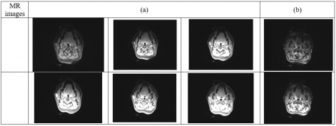
All MRI examinations were performed with a dedicated head and neck coil, with a Signa model HDxt 3-T (Tesla) machine (GE Healthcare). T1-MR sequences were obtained after an intravenous injection of contrast material (gadopentetate dimeglumine). The parameters for the T1-weighted sequence were TR-TE=6.8-1.2, with 256 x 256 matrix, maximum voxel resolution of mm3. The employed sequences present images in each one having 256 grey levels and pixels for each image. Similarly, the device and the computer specification resolutions were respectively (inchs) and (pixels). Figure 1 exposes some examples of MR images.
2.2 Description of the proposed method
In the clinical examination, the PG lesions were completely determined by different experts. Nevertheless, the biometric measurements (ROI size, perimeter...) are not adequate enough to distinguish the large variation of PG lesion. In this paper, a new automatic region of interest (ROI) detection method combined with pertinent classification scheme is proposed for PG status.
Figure 1. T1-MRI examples of eight images: (a) PG lesion cases and (b) Normal cases
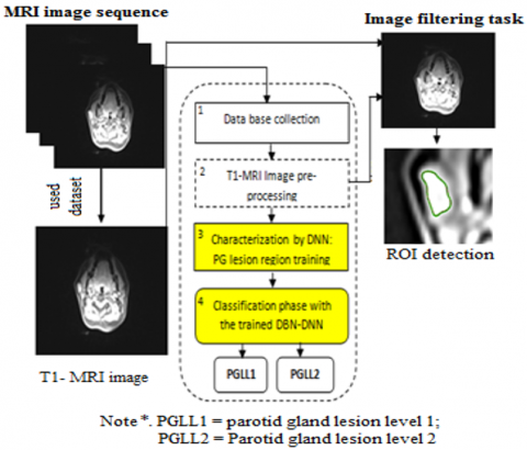
In this work, an advanced classification scheme combined with applicable textural region characteristics is proposed. The first tasks of the proposed method were presented in our previous work [28]. In this contribution, a continuation of the proposed work [13] is presented where widely of information are treated to obtain effective performances in images denoising scheme. The proposed method [28] is included a chief part. Different images pre-processing strategy is first applied by the use of filtering technique to reduce the noise in used images. Second strategy, appreciated parotid gland segmentation is achieved to detect the lesion region based on the GAC. Figure 2 summarizes the overall stages of the proposed analysis scheme.
Figure 2. The proposed methodology
Hence, the contribution of this work is divided into two principle folds:
• MR Images segmentation: Appreciated Parotid gland lesion segmentation is achieved to detect the region of interest based on the GAC.
• Intelligent Classification framework: An image categorization strategy is projected in order to classify the MR subjects into two groups: parotid gland lesion level 1 (PGLL1) and parotid gland lesion level 2 (PGLL2) datasets. The Deep Neural Network (DNN) method is applied for classification step. Here, the previous detection results of PG lesion boundary are employed to characterize the anomaly using T1-MR images [13]. The DNN model classifier is performed to recognize MR images in different cases. This method is primarily recipient for precocious detection of PG defect progression using early period assessment.
2.2.1 Image pre-processing Stage using BM3D technique
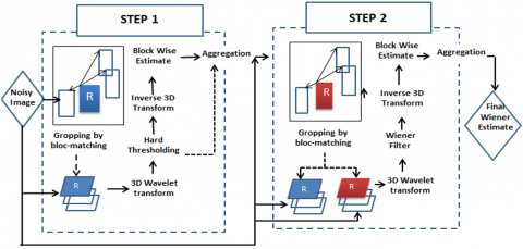
In this phase, a filtering method based on BM3D algorithm is implemented to improve the image quality and facilitate subsequent work steps. The main structure of the BM3D algorithm can be split into two major steps. The first step estimates the de-noised image using hard thresholding during the collaborative filtering and can be divided into three sub-steps. These sub-steps start by finding the image patches P(P) similar to given ones and grouping them into a 3D block, then a 3D linear Wavelet transform and shrinkage of coefficient are applied to these blocks. Finally, an inverse 3D transform is applied using the following equation.
$P(P)^{\text {hard }}=\tau_{3 D}^{\text {hard }-1}\left(\gamma\left(\tau_{3 D}^{\text {hard }}(P(P))\right)\right)$ (1)
where, γ is a hard thresholding operator with threshold $\lambda_{3 D}^{\text {hard }} \sigma$ such as σ designates the zero means Gaussian noise variance.
$\gamma(x)= \begin{cases}0 & \text { if }|x| \leq \lambda_{3 D}^{\text {hard }} \sigma \\ x & \text { otherwise }\end{cases}$ (2)
The final 3D block consists of the simultaneously filtered 2D image patches. The last step is the aggregation operation it gives an estimate for each used patch. These estimates are saved in a buffer.
$\forall Q \in P(P), \forall x \in Q,\left\{\begin{array}{l}v(x)=v(x)+w_{P}^{h a r d} \mu_{Q, P}^{h a r d}(x) \\ \delta(x)=\delta(x)+w_{P}^{h a r d}\end{array}\right.$ (3)
where:
- ν and δ designate respectively the numerator and the denominator part of the basic estimate of the image obtained at the end of the grouping step
- $u_{Q, P}^{\text {hard }}$ designate the estimate of the value of the pixel x obtained during collaborative filtering.
$w_{P}^{\text {hard }}= \begin{cases}\left(N_{p}^{\text {hard }}\right)^{-1} & \text { if } N_{p}^{\text {hard }} \geq 1 \\ 1 & \text { otherwise }\end{cases}$ (4)
Such as $N_{P}^{\text {hard }}$ refer to the non-zero coefficients in the 3D block obtained after hard thresholding mentioned above.
The obtained basic estimate after this first step is given by the following equation.
$u^{\text {basic }}(x)=\frac{\sum_{P} w_{P}^{\text {hard }} \times \sum_{Q \in P(P)} \quad \chi Q(x) u_{Q, P}^{\text {hard }} \quad (x)}{\sum_{P} w_{P}^{h a r d} \quad \times \sum_{Q \in p(P)} \quad \chi Q(x)}$ (5)
This estimate is simply obtained by dividing the two buffers, which are the numerator and the denominator, element by element with respect to the following condition.
$\chi Q(x)= \begin{cases}1 & \text { if and only if } x \in Q \\ 0 & \text { otherwise }\end{cases}$ (6)
The second main step is carried out by using Wiener filtering. This second step imitates the first one with two differences taken into account [2]. The filtered patches are compared instead of the original patches. The new 3D group is processed by Wiener filtering instead of a simple threshold.
Three sub steps are carried out in this stage: designated grouping, collaborative filtering, and aggregation. During the grouping operation, the patch-matching is handled on the basic estimate $u^{\text {basic }}$. In fact, a set of similar patches are collected to form 3D groups.
$P^{\text {basic }}(P)=\left\{Q: d(P, Q) \leq \tau^{\text {wiener }}\right\}$ (7)
where:
- $P^{\text {basic }}(P)$ and P(P) are respectively obtained after the stacking of the similar patches from the basic estimate and the original noisy image.
- $\tau^{\text {wiener }}$ is the distance threshold for d under which two patches are assumed similar.
After the grouping operation, which is achieved by finding the 3D blocks, the collaborative filtering can be started. The filtering operation of P(P) called Wiener collaborative filtering is achieved by using Wiener filtering. In fact, the resulting image is produced by multiplying element by element the 3D transform of the noisy image with the Wiener coefficients defined as follow.
$w_{p}(\xi)=\frac{\left|\tau_{3 D}^{\text {wien }}\left(P^{\text {basic }}(P)\right)(\xi)\right|^{2}}{\left|\tau_{3 D}^{\text {wien }}\left(P^{\text {basic }}(P)\right)(\xi)\right|^{2}+\sigma^{2}}$ (8)
The estimate of the 3D group is obtained by the Eq. (9).
$P^{\text {wien }}(P)=\tau_{3 D}^{\text {wien }^{-1}}\left(w_{P} . \tau_{3 D}^{\text {wien }}(P(P))\right)$ (9)
The last minor step is the aggregation which takes place when the collaborative filtering is achieved. This step aims to store in a buffer the estimate for every pixel.
$\forall Q \in P(P), \forall x \in Q,\left\{\begin{array}{l}v(x)=v(x)+w_{P}^{\text {vien } } u_{Q, P}^{\text {wien }}(x) \\ \delta(x)=\delta(x)+w_{P}^{\text {wien }}\end{array}\right.$ (10)
where:
- τ and δ designate respectively the numerator and the denominator part of the final estimate image which is obtained in the end of the first step.
- $u_{Q, P}^{\text {wien }}(x)$ is the estimation of the value of the pixel x belonging to the patch Q obtained during the collaborative filtering of the reference patch P.
$w_{P}^{\text {wien }}=\left\|w_{P}\right\|_{2}^{-2}$ (11)
The final estimate image is given according to the Eq. (12):
$u^{f_{\text {inal }}}(x)=\frac{\sum_{P} w_{P}^{\text {wien }} \sum_{Q \in P(P)} \quad \chi Q(x) u_{Q, P}^{\text {wien }} \quad (x)}{\sum_{P} w_{P}^{\text {wien }} \sum_{Q \in P(P)} \quad \chi Q(x)}$ (12)
Following the first major step, the final estimate is simply obtained by dividing the two buffers, which are the numerator and the denominator, element by element with respect to the condition mentioned in Eq. (12).
All these steps are summarized in the Figure 3.
Figure 3. Diagram of the BM3D algorithm
2.2.2 PG lesion boundary detection
The objective of the first stage of the proposed automatic PG lesion segmentation technique is the boundary contour extraction of the lesion region from the remainder (background). This task is based on a geodesic active contour model initialized by an elliptic curve that estimates the lesion region in the PG.
The GAC approach [29] is applied to segment the object edge in a grayscale image by finding a curve C that decrease the following energy function:
$E_{C}(C)=\int_{0}^{L(C)} g(C(q)) d s+v \int_{\Omega} g(C(q)) d A$ (13)
where, $C(q)=(x(q), y(q)$, is a curve in Ω with a position parameter $q \in[0,1]$ and L represents the Euclidean distance. The distance ds is the Euclidean metric, dA is the parameter of area and v is a parameter which controls the area of the active contour. Ωϵ$R^{2}$ is the 2D space of the gray level image, and g is the stopping function of the curve (edge-detector) for gray image. The progress of the curve is controlled by the stopping function represented by the following form:
$g=\frac{1}{1+\left|\nabla\left(G_{\sigma} * I\right)\right|}$ (14)
where, I is the image intensity and G represents the Gaussian kernel. The curve is categorized by two parameters the normal direction N with a convergence parameter F:
where, Gσ is the Gaussian kernel with standard deviation σ. The curve is characterized by two parameters; the normal direction N with speed convergence F:
$\frac{\partial C(t)}{\partial t}=F . \overrightarrow{\mathrm{N}}$ (15)
The level set method, introduced by Osher and Sethian [19] to find a numerical solution of this problem (Eq. (1)), consists on representing the contour C(t) as being the zero level of two dimensional Lipchitz continuous function ϕ(p, t), called the level set function. In other words, the contour C(t) is the set of points P(x, y) such as:
$C(t)=\{p / \phi(p, t)=0\}$ (16)
where, ϕ is the signed distance function that gives the location of a point p with respect to the contour C:
$\phi(p)= \begin{cases}+d, & p \text { is outside } C \\ 0, & p \text { in } C \\ -d & p \text { is inside } C\end{cases}$ (17)
The level set function ϕ for the contour point must have the zero value at each time:
$\phi(C(t), \mathrm{t})=0$ (18)
The derivative of the level set function is given by:
$\frac{\partial \phi(C(t), t)}{\partial t}=\frac{\partial \phi(C(t), t)}{\partial t}+\frac{\partial \phi(C(t), t)}{\partial C} \cdot \frac{\partial C}{\partial t}=0$ (19)
The Eq. (19) is written as:
$\frac{\partial \phi}{\partial t}+\nabla \phi \cdot \frac{\partial C}{\partial t}=0$ (20)
From the Eq. (19), the gradient of ϕ function represents the normal N vector of the contour and the evolution rate is a direction normal to the curve:
$F=\frac{\partial C}{\partial t} . \vec{N}$ (21)
The Eq. (15) is integrated in (20), and, we obtain the evolution equation given by:
$\frac{\partial \phi}{\partial t}+F .\|\nabla \phi\|=0$ (22)
The curve evolution is generally a function of the image and the curve characteristics [30]. The original formulation of the GAC model [19] is given by:
$\frac{\partial \phi}{\partial t}=g(\kappa+v) .\|\nabla \phi\|$ (23)
where, the product g(κ+ν) fixed the evolution speed of level sets of ϕ(p, t) along their normal direction and κ is the curvature which is used here to accomplish the smoothness of the contour.
The curvature is given by [17]:
$\kappa=\operatorname{div}\left(\frac{\nabla \phi}{\|\nabla \phi\|}\right)=\frac{\phi_{x x} \phi_{y}^{2}-2 \phi_{x} \phi_{y} \phi_{x y}+\phi_{y y} \phi_{x}^{2}}{\left(\phi_{x}^{2}+\phi_{y}^{2}\right)^{3 / 2}}$ (24)
The mathematical curve solution of the curve evolution problem is given by the fast level set formulation proposed in [30]:
$\left\{\begin{array}{l}\frac{\partial \phi}{\partial t}=\delta_{\varepsilon}(\phi)\left(\lambda \operatorname{div}\left(g \frac{\nabla \phi}{|\nabla \phi|}\right)+v g\right)+\mu \operatorname{div}((1-1 /|\nabla \phi|) \nabla \phi) \\ \phi(x(t), y(t), 0)=\phi^{0}(x(t), y(t))\end{array}\right.$ (25)
m is a positive parameter that controls the penalization term $\operatorname{div}((1-1 /|\nabla \phi|) \nabla \phi$ which is applied to fix the level set function close to the signed distance function during the curve evolution (see [17]). Where λ presents a constant controlling the curvature term and $\delta_{\varepsilon}(\phi)$ is a parameter that regularizes the Dirac function with a width controlled by e [17]. $\phi^{0}(x, y)$ is the initial contour in each frame of the MR images.
Finally, the discrete level set function is given by:
$\phi^{k+1}(x, y)=\phi^{k}(x, y)+\tau L\left(\phi^{k}(x, y)\right)$ (26)
where, $L\left(\phi^{k}(x, y)\right.$ presents the approximation of the right-hand side in (24) and τ is the time step.
The initial curve is constructed by an ellipse mask selected with five ellipse parameters (xc, yc, a, b, θ) where $x_{c}$ and, $y_{c}$ represent the circle centroid, the two ellipse radius (a, b) and θ is to the ellipse angle, which are achieved from the Otsu segmentation method [31]. The idea of this latter method is to detect the PG lesion before the initialization of GAC model. Since the PG presents a low grayscale level, a maximum intensity value is fixed as a threshold based on minimizing the intra-class variance and maximizing the ratio between the interclass variance and the total variance, each frame segmented is composed of two different regions: the region of interest ROI (the Lesion in PG) and the background. Here, to speed up the convergence of the GAC algorithm, we optimized the number of iterations of the curve evolution using the ellipse fitting error. The relative function of error $f_{\text {iter }}$ is computed as follow:
$f_{\text {iter }}=\frac{\text { cover }_{\text {ellip }}-\text { Lesion }_{\text {rough }}}{\text { Lesion }_{\text {rough }}} \times 100$ (27)
where, coverellip represents the area that the initial ellipse covers, and the Lesionrough is the rough lesion area obtained by fixed thresholding. The iteration number noted Iter was computed and reduced as given in the following equations:
iter $=20$ if $\quad f_{\text {iter }} \leq 0.09$ (28)
iter $=30$ if $0.09 \leq f_{\text {iter }} \leq 0.12$ (29)
For the analysis of subsequent MR image frames, the lesion region is chosen based on the current frame segmentation result. In fact, to remove the influence of background artifacts and to limit the computation time of the contour evolution, the initial curve is detected based on the current result.
2.2.3 Classification of PG lesion using DBN-DNN classifier
In this study, the deep neural network method is realized in order to classify the extracted PG lesion boundary and to distinguish between PG lesion levels (level 1 and level 2). Several classification methods can be employed for pattern recognition. Nevertheless, for multiple categorization works [32, 33], it has been confirmed that DNN presents a high-quality tool. To acquire authentic classification results, we have selected the PG region of different images for assembling the training dataset of the network. Consequently, both learning and training neural network stage are performed using the morphological information (texture, area…) of PGs lesion region.
The DNN classification phase is composed into two diverse tasks: (i) the training task that included the greater part of the database (184 subjects randomly chosen using two cases (PGLL1 and PGLL2) which allow the learning and the training of the network. At the same time as (ii) the test task is reserved to validation part that involved the smaller part of the database (the remaining subjects: 122 subjects) taking into account that the examples of the validation set do not belong to the training set. In addition, applying the back-propagation (BP) algorithm, the network is learned with conjugate gradient training method [34, 35].
The neural network structure is composed of two inputs classes, are either (0.95) for (PGLL1), (-0.95) for (PGLL2). In this network, the hyperbolic tangent sigmoid transfer function is applied for all neurons as activation function. The maximum number of iterations (20 epochs of training) is reached or the mean square error (MSE) is decreases to a mean of 8.10-2.
To improve classification results, all previous works have focused their diagnosis on visual inspection of segmented PG lesion region. The superiority of this study is highlighted by the use of detected ROI by some customized processing tools, and the use of the classification technique using deep learning strategy which was not detained before.
(1) Classification using deep neural network
In this study, the DBN-DNN method is performed to differentiate between two categories of parotid gland lesions. Yet, for numerous classification works [36, 37], it has been proved that DNN represents a high quality methodology for pattern recognition. The deep learning step of the network is performed using PG lesion characteristics. Taking into account the similarity between the characteristics of different PG tumor regions, the DNN procedure is considered using the feature number in the input learning set to obtain the most discriminative features distorted to a suitable illustration of the database used (1×(2 output classes)).
The deep learning step of the network is performed using image feature vectors. Taking into account the resemblance between different characteristics extracted from each PG class in the MR image, the DBN-DNN procedure uses a number of features in the input learning set to obtain the most discriminative characteristics.
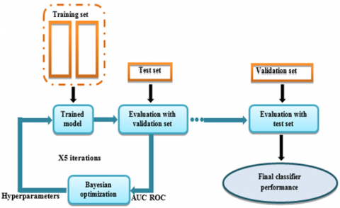
The cross-validation experiment is used to give the best DBN-DNN structure. The training-segment vectors sets are divided into five equally-sized sub datasets (five folds). Each iteration contains four folds for the training and one fold for the validation. The tangent sigmoid transfer function is applied for all neurons. Five iterations are achieved for the training and validation phase. After the selection of the hyper parameters, the DBN-DNN classifier was trained and evaluated using the test set (see Figure 4).
Figure 4. Diagram of the cross-validation and the optimisation process
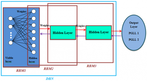
Figure 5. The structure of the DBN classifier
(2) Constructing the DBN classifier
The architecture of the DBN classifier is shown in Figure 5, which is composed of three RBMs (RBM1, RBM2 and RBM3) and an output layer which presents the two PG’s lesion levels (PGLL 1 and 2). Firstly, we have to train in an unsupervised way in order to train the DBN classifier. Then, the trained DBN is also combined with the output layer to form the input of the deep neural network (DNN). The DBN is obtained and the DNN is trained by the back-propagation (BP) algorithm in a supervised way.
(3) Training DBN with RBMs
1) Training restricted Boltzmann machine (RBM)
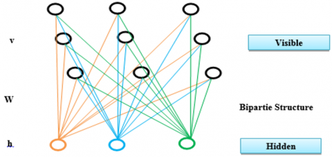
A restricted Boltzmann machine (RBM) is a specific type of random neural network design that has two-layer architecture. The first input layer is called visible layer, where the second layer is called hidden layer. Between two layers, nodes are fully connected, nevertheless in the same layer there is no connection. Though, we constitute a bipartite structure. Figure 6 shows that the bottom layer contains visible variables (nodes) and the top layer contains hidden variables (nodes). The symmetric interaction terms between the visible variables and the hidden variables are represented by the matrix W.
Figure 6. The structure of the RBM
The energy function of the joint configuration can be defined by:
$E(v, h ; \theta)=-\sum_{i j} W_{i j} \nu_{i j} h_{j}-\sum b_{i} v_{i}-\sum a_{j} h_{j}$ (30)
where, $\theta=\{W, a, b\}$ represents the model parameters, $a_{i}$ is the bias of visible unit i, and $b_{i}$ is the bias of hidden unit j.
The joint probability distribution of a certain configuration is achieved by the Boltzmann distribution (and the energy of this configuration):
$P_{\theta}(v, h)=\frac{1}{Z(\theta)} \exp (-E(v, h ; \theta))$ (31)
where, Z(θ) is the normalization constant.
If ν=(v1, v2, …, vi) is an input vector to the visible layer, the binary state $h_{j}$ of the hidden unit j is fixed to 1 with the probability as follows:
$P\left(h_{j}=1 \mid v\right)=\operatorname{sigmoid}\left(\sum_{i} W_{i j} v_{i}+a_{j}\right)$ (32)
With the states of the hidden units, the binary state $v_{i}$ of visible unit i is set to 1 with the probability below:
$P\left(v_{i}=1 \mid h\right)=\operatorname{sigmoid}\left(\sum_{j} W_{i j} h_{j}+b_{i}\right)$ (33)
The RBM structure is frequently trained as follows:
This section summarizes the T1-MR image filtering, segmentation and classification results. In addition, due to the classification stage has not been mentioned in other works [38, 39], this study offers a vital and an attractive ability to categorize pathological data related to the degree of malignity (PGs Lesion level 1 or PGs Lesion level 2). All experiments are verified with those evaluated by experts in term of PG lesion boundary segmentation assignment. Three experts, with diverse expertise degrees, participated in defining the different lesion ground truth at two different statuses, however, segmentation approach was provided independently for each expert. The resulting manual delineations have no relationship with expertise degrees of Experts.
3.1 Results of T1-MR image filtering
The BM3D technique is studied to realize an accuracy regarding shape’s continuity and noise removal. The proposed filtering methods are displayed in Figure 7 to reveal the proposed denoising strategy using the same dataset. Hence, the performance of the employed method is validated by the evaluation criteria using the Signal-to-Noise Ratio (SNR) and the Peak Signal-to-Noise Ratio (PSNR) measures.
Figure 7. Overview of the BM3D filtering results
Therefore, the performance of the employed method is validated using the Peak Signal-to-Noise Ratio (PSNR) and the Signal-to-Noise Ratio (SNR) measures. Here, we noticed that the proposed methodology provides the mean of SNR (11.05db) and PSNR (about 31.25 db) values for the 30 MR images datasets. Therefore, compared to the work of [40], the effectiveness of proposed algorithm was determined with promised filtering results reducing efficiently the remarkable noise in view of MRI dataset.
3.2 Results of PG lesion detection
In this section, we present the PG detection results using the GAC model. In Figure 8, we show the fixed blue ellipse that corresponds to the initial mask, established by the MR frames.
Indeed, the main idea of the proposed GAC procedure is to extract the PG lesion region in each frame of the MR images before the initialization of GAC model.
To extract edges of the desired PG lesion from background of the processed frame, we used the level set function using the proposed GAC model. In addition, Figure 8 reveals the evolution of GAC model in an extracted MR image using maximum of 30 iterations. In order to prove the performance of our method in lesion detection on the MRI database, we choose 6 images representing two lesion levels (level 1 and level 2). Besides, a good performance of these active contours is achieved by an automatic estimation of final curves when compared to experts.
Figure 8. PG lesion contour detection results using the proposed GAC algorithm of three MR images
Essentially, the proposed GAC algorithm was tested on 54 frames randomly chosen from the MRI database compared to the manually segmentation results given by Experts. The region measure is used to offer the difference between the edge detection region (BR) and the ground-truth regions (GTR) segmented manually by doctors.
The evaluation measures used in this work is the region accuracy (RA) can be represented as follow:
$R A(\%)=100 \times\left[1-\frac{[A(B R) \cup A(G T R)]-[A(B R) \cap A(G T R)]}{[A(B R) \bigcup A(G T R)]}\right],$ (34)
where, A (BR) and A (GTR) present respectively the segmented regions areas (BR) and (GTR). As shown in Table 1, the performance of the proposed GAC model is compared to ground truth given by experts from MR image results. As mentioned, the performance of the PG lesion detection algorithm usually depends on the trade-off between rapidity and accurateness.
Here, a statistical metrics such as: Mean, min, standard deviations, max and times of convergence are applied for the evaluation of the detection method performance. The average of these performance measures in terms of region segmentation accuracies using 30 images dataset is computed, leading to 97.35% of accuracy with a standard deviation about 2.74. For the used MRI data sets, the proposed methodology is clearly hopeful in terms of region segmentation accuracies. Also, the performance of the proposed GAC algorithm is qualitatively compared to the ground truth. DSC and JC are respectively about an average of 93.54% and 92.89% using the GAC model. Furthermore, it gives a rapid mean convergence speed (about 1 second for each frame to detect the lesion boundary).
Table 1. Comparison of PG lesion segmentation results using GAC method in term of ROI detection on MRI
|
|
|
The proposedGACmethod |
|
Accuracy (%) |
Mean |
97.35 |
|
Standard deviation |
2.74 |
|
|
Min |
86.75 |
|
|
Max |
98.05 |
|
|
|
Dice |
93.54 |
|
|
Jaccard |
92.89 |
|
Total time of convergence (s) |
1.24 |
|
3.3 PG lesion classification results
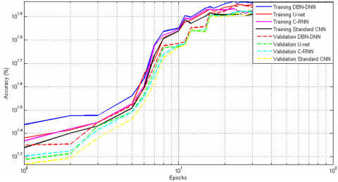
PG lesions classification stage aims to create a significant separation of subjects into two classes related to the degree of lesion progress (lesion level 1 or lesion level 2) in order to improve the diagnostic of PG anomalies. The deep learning process is divided into two important steps: The training and the validation. The resulting accuracies demonstrate the superiority of DBN-DNN proposed classifier when compared to the U-net, C-RNN, and standard CNN methods. From the obtained results revealed in Table 2, it is clear that the DNN classifier is more effective in term of the highest accuracy rate with an average of 91.76.
The obtained classification rate presents the highest precision when compared with the tested approaches. Besides, the proposed methodology supplied an effectual characterization phase of the most appropriate information clearly distinguished the two levels of PG lesion (PGLL1, PGLL2). The establishment of a PG diagnosis can be considered as a binary decision which can be divided into four distinct situations (See Table 3).
To enhance our comparative study, ROC parameters are evaluated in this section. ROC measures are given by [42]:
The accuracy classification (AC) is the ratio of the total numbers of correctly classified test samples to the total number of test samples.
$A C=\frac{T P+T N}{T P+F N+T N+F P}$ (35)
The sensitivity (SE) of a diagnostic test is the number of subjects for whom the result is positive that are correctly identified by the test.
$S E=\frac{T P}{F N+T P}$ (36)
The specificity (SP) is the class of subjects for whom the result is negative that are correctly identified by the test.
$\mathrm{SP}=\frac{\mathrm{TN}}{\mathrm{TN}+\mathrm{FP}}$ (37)
where, TP and TN represent respectively the number of true positives and true negatives, FP is the number of false positives and FN is the number of false negatives.
To significantly explain the used parameters of different compared methods [41], Table 4 is perceptibly established to summarize the employed hyper-parameters in the resulting classification strategies.
The proposed strategy offers important recognition results in view of statistical evaluations (AC, SE and SP) with a mean average of 92.15%, 91.36% and 93.51%, respectively. Compared to different deep learning techniques, the proposed procedure completes a capable classification of MR images dataset and clearly distinguished the two parotid gland levels.
Figure 9 presents the ROC curve to approve the experimental classification results. Then, in order to select the best classifier, a common method that can be used here is to compute the area under the ROC curve. The value of this area is fixed between 0 and 1 and it corresponds to the value 1 for an ideal classifier. In this work, the area under curves is equal to 0.87, 0.84, 0.79, and 0.76 for DNN, U-net, C-RNN and standard CNN respectively.
Figure 9. Training and validation performances using our proposed DBN-DNN model compared to U-net, C-RNN and standard CNN applied on MRI datasets for two classes
Table 2. A comparison between previous studies and the current study
|
Standard CNN |
C-RNN |
U-net |
The proposedDBN-DNN method |
|
|
Fold 1 |
81.54 |
84.67 |
88.72 |
92.82 |
|
Fold 2 |
79.47 |
85.25 |
88.33 |
91.44 |
|
Fold 3 |
80.15 |
83.49 |
87.45 |
92.98 |
|
Fold 4 |
79.14 |
81.76 |
89.04 |
91.03 |
|
Fold 5 |
77.69 |
83.35 |
87.23 |
90.55 |
|
Mean |
79.60 |
83.70 |
88.15 |
91.76 |
Table 3. Parotid Gland tumor diagnostic tests
|
|
Patients |
*Note: PGLL1: Parotid Gland Lesion L1 PGLL2: Parotid Gland Lesion L2 TP: True Positive TN: True Negative FP: False Positive FN: False Negative |
||
|
Effectively L1 |
Effectively L2 |
|||
|
Observer response |
PGLL1 |
TP |
FP |
|
|
PGLL2 |
FN |
TN |
||
Table 4. A detailed process for comparison with standard CNN, C-RNN and U-net methods
|
|
|
Proposed method |
||
|
Classifiers |
Standard CNN |
C-RNN |
U-net |
DBN-DNN |
|
Epoch |
20 |
20 |
20 |
20 |
|
Training method |
SBP |
SBP |
SBP |
SBP |
|
Neighbor number |
- |
- |
- |
- |
|
Distance function |
- |
- |
- |
- |
|
Threshold |
- |
- |
- |
- |
|
Activation function |
Tan-Sig |
Pretanh |
Tan-Sig |
Tan-Sig |
|
SP |
81.29 |
84.34 |
90.06 |
93.51 |
|
SE |
81.06 |
82.69 |
89.65 |
91.36 |
|
AC (%) |
79.98 |
83.56 |
88.14 |
92.15 |
*Note: SBP:Standar Back,Parametric rectified tanh : Pretanh , Tan-Sig: Tangent Sigmoid transfert function.
Table 5. Summary of some studies reporting PG lesion diagnosis
|
Literature |
Year |
Used technique |
Used Dataset |
Dice (%) |
PG Lesion Classification Accuracy |
|
Yang et al. [38] |
2014 |
Statistical features+ SVM |
MRI |
90.5 |
- |
|
Močnik et al. [39] |
2018 |
CNN multimodal segmentation |
CT+MRI |
78.7 |
- |
|
Hänsch et al. [40] |
2018 |
U-net segmentation |
CT |
88 |
- |
|
Proposed method |
- |
GAC+ (DBN-DNN) |
MRI |
93.54 |
92.15 |
3.4 Discussion and comparison with some previous works
The majority of existing segmentation methods use atlas software as an integral part, of prior segmented images, and the propagated atlas images are then used as a basis for further segmentation enhancement, using statistical shape, active contours and appearance models. Nevertheless, in the work of Yang et al. [38], multiple features from subject-specific atlas pairs were used to train the kernel SVM based on RBF kernel. The proposed segmentation method could robustly differentiate the parotid tissue from surrounding tissues by statistically matching multiple texture features. However, this study needs to test the sensitivity of multiple features in order to decreasing the number of feature numbers. The proposed study [39] using CNN method gives pertinent segmentation results of tumors and the segmentation methodology does not require a learning process. However, its definition is inconsistent. In some cases, this method may not completely cover some structures, and indicates an insufficient ability to fill some portions of the structure with non-negligible surface area. In the work of Hänsch et al. [40], authors presented a strategy of parotid gland detection using multimodal U-net architecture, the segmentation results are significantly better than those given by atlas-based methods. This demonstrates the high potential of deep learning-based segmentation methods for radiotherapy arrangement. However the learned features need to be trained on a larger dataset. As shown in Table 5, the segmentation accuracies of the proposed GAC method presents effective segmentation accuracies when compared with other considered methods from the literature. Evaluation measures of the proposed segmentation and classification approaches of PG lesion levels compared to other existing methods are presented in Table 5.
This paper deals a completely automatic method that can be applied for parotid gland lesion detection in different level of malignity in MR images. First, a consecutively pre-process model based on a BM3D technique was used to MR images filtering in order to improve the original image quality. The proposed method gives finest approach for parotid gland ROI detection. Second, a Geodesic active contour model was employed to PG lesion detection. Then to classify the MR images into two categories: PG lesion level 1 or 2 using the deep network classifier. The proposed methodology frequently supports a hard groundwork for computer-assisted anomalies evaluation system of an expert early diagnosis. In future work, we can develop deep classification methods for training networks using more large training data, by replicating and modifying existing samples to generate new dataset.
[1] Bray, F., Ferlay, J., Soerjomataram, I., Siegel, R.L., Torre, L.A., Jemal, A. (2018). Global cancer statistics 2018: GLOBOCAN estimates of incidence and mortality worldwide for 36 cancers in 185 countries. CA: A Cancer Journal for Clinicians, 68(6): 394-424. https://doi.org/10.3322/caac.21492
[2] Delaney, G.P., Barton, M.B. (2015). Evidence-based estimates of the demand for radiotherapy. Clinical Oncology, 27(2): 70-76. https://doi.org/10.1016/j.clon.2014.10.005
[3] Hawkins, P.G., Lee, J.Y., Mao, Y., Li, P., Green, M., Worden, F.P., Eisbruch, A. (2018). Sparing all salivary glands with IMRT for head and neck cancer: Longitudinal study of patient-reported xerostomia and head-and-neck quality of life. Radiotherapy and Oncology, 126(1): 68-74. https://doi.org/10.1016/j.radonc.2017.08.002
[4] Wang, L.W., Liu, Y.W.H., Chou, F.I., Jiang, S.H. (2018). Clinical trials for treating recurrent head and neck cancer with boron neutron capture therapy using the Tsing-Hua Open Pool Reactor. Cancer Communications, 38(1): 1-7.
[5] Yang, L., Lu, J., Dai, M., Ren, L. J., Liu, W. Z., Li, Z.Z., Gong, X.H. (2016). Speckle noise removal applied to ultrasound image of carotid artery based on total least squares model. Journal of X-ray Science and Technology, 24(5): 749-760. https://doi.org/10.3233/XST-160570
[6] Zhang, Y., Salehjahromi, M., Yu, H. (2019). Tensor decomposition and non-local means based spectral CT image denoising. Journal of X-ray Science and Technology, 27(3): 397-416. https://doi.org/10.3233/XST-180413
[7] Tebini, S., Mbarki, Z., Seddik, H., Braiek, E.B. (2016). Rapid and efficient image restoration technique based on new adaptive anisotropic diffusion function. Digital Signal Processing, 48: 201-215. https://doi.org/10.1016/j.dsp.2015.09.013
[8] Seo, H.U., Wei, Q., Kwon, S.G., Sohng, K.I. (2017). Medical image watermarking using bit threshold map based on just noticeable distortion in discrete cosine transform. Technology and Health Care, 25(S1): 367-375. https://doi.org/10.3233/THC-171340
[9] Isa, I.S., Sulaiman, S.N., Mustapha, M., Darus, S. (2015). Evaluating denoising performances of fundamental filters for T2-weighted MRI images. Procedia Computer Science, 60: 760-768. https://doi.org/10.1016/j.procs.2015.08.231
[10] Kaur, P., Singh, G., Kaur, P. (2018). A review of denoising medical images using machine learning approaches. Current Medical Imaging, 14(5): 675-685. https://doi.org/10.2174/1573405613666170428154156
[11] Handayani, A., Suksmono, A.B., Mengko, TL., Hirose, A. (2012). Blood vessel segmentation in complex-valued magnetic resonance images with snake active contour model. In Emerging Communication Technologies for E-Health and Medicine (pp. 196-207). IGI Global. https://doi.org/10.4018/978-1-4666-0909-9.ch015
[12] Agner, S.C., Xu, J., Madabhushi, A. (2013). Spectral embedding based active contour (SEAC) for lesion segmentation on breast dynamic contrast enhanced magnetic resonance imaging. Medical Physics, 40(3): 032305. https://doi.org/10.1118/1.4790466
[13] Li, Y., Cao, G., Wang, T., Cui, Q., Wang, B. (2020). A novel local region-based active contour model for image segmentation using Bayes theorem. Information Sciences, 506: 443-456. https://doi.org/10.1016/j.ins.2019.08.021
[14] Ma, C., Luo, G., Wang, K. (2018). Concatenated and connected random forests with multiscale patch driven active contour model for automated brain tumor segmentation of MR images. IEEE Transactions on Medical Imaging, 37(8): 1943-1954. https://doi.org/10.1109/TMI.2018.2805821
[15] Slama, A.B., Mouelhi, A., Sahli, H., Manoubi, S., Mbarek, C., Trabelsi, H., Sayadi, M. (2017). A new preprocessing parameter estimation based on geodesic active contour model for automatic vestibular neuritis diagnosis. Artificial Intelligence in Medicine, 80: 48-62. https://doi.org/10.1016/j.artmed.2017.07.005
[16] Mouelhi, A., Sayadi, M., Fnaiech, F., Mrad, K., Romdhane, K.B. (2013). Automatic image segmentation of nuclear stained breast tissue sections using color active contour model and an improved watershed method. Biomedical Signal Processing and Control, 8(5): 421-436. https://doi.org/10.1016/j.bspc.2013.04.003
[17] Zheng, Y., Li, G., Sun, X., Zhou, X. (2009). A geometric active contour model without re-initialization for color images. Image and Vision Computing, 27(9): 1411-1417. https://doi.org/10.1016/j.imavis.2009.01.001
[18] Yu, H., He, F., Pan, Y. (2018). A novel region-based active contour model via local patch similarity measure for image segmentation. Multimedia Tools and Applications, 77(18): 24097-24119.
[19] Osher, S., Paragios, N. (Eds.). (2003). Geometric level set methods in imaging, vision, and graphics. Springer Science & Business Media. https://doi.org/10.1007/b97541
[20] Mangoubi, O., Smith, A. (2018). Rapid mixing of geodesic walks on manifolds with positive curvature. Annals of Applied Probability, 28(4): 2501-2543. https://doi.org/10.1214/17-AAP1365
[21] Li, C., Xu, C., Gui, C., Fox, M.D. (2005). Level set evolution without re-initialization: A new variational formulation. In 2005 IEEE Computer Society Conference on Computer Vision and Pattern Recognition (CVPR'05), 1: 430-436. https://doi.org/10.1109/CVPR.2005.213
[22] Schupp, S., Elmoataz, A., Fadili, J., Herlin, P., Bloyet, D. (2000, September). Image segmentation via multiple active contour models and fuzzy clustering with biomedical applications. In Proceedings 15th International Conference on Pattern Recognition. ICPR-2000, IEEE, 1: 622-625. https://doi.org/10.1109/ICPR.2000.905415
[23] Torfeh, T., Hammoud, R., Perkins, G., McGarry, M., Aouadi, S., Celik, A., Al-Hammadi, N. (2016). Characterization of 3D geometric distortion of magnetic resonance imaging scanners commissioned for radiation therapy planning. Magnetic Resonance Imaging, 34(5): 645-653. https://doi.org/10.1016/j.mri.2016.01.001
[24] Özyurt, F., Sert, E., Avci, E., Dogantekin, E. (2019). Brain tumor detection based on Convolutional Neural Network with neutrosophic expert maximum fuzzy sure entropy. Measurement, 147: 106830. https://doi.org/10.1016/j.measurement.2019.07.058
[25] Li, Y., Dai, Y., Yu, N., Duan, X., Zhang, W., Guo, Y., Wang, J. (2019). Morphological analysis of blood vessels near lung tumors using 3-D quantitative CT. Journal of X-ray Science and Technology, 27(1): 149-160. https://doi.org/10.3233/XST-180429
[26] Belal, S.L., Sadik, M., Kaboteh, R., Enqvist, O., Ulén, J., Poulsen, M. H., Trägårdh, E. (2019). Deep learning for segmentation of 49 selected bones in CT scans: First step in automated PET/CT-based 3D quantification of skeletal metastases. European Journal of Radiology, 113: 89-95. https://doi.org/10.1016/j.ejrad.2019.01.028
[27] Pi, L., Shen, C., Li, F., Fan, J. (2007). A variational formulation for segmenting desired objects in color images. Image and Vision Computing, 25(9): 1414-1421. https://doi.org/10.1016/j.imavis.2006.12.013
[28] Mbarki, Z., Seddik, H., Tebini, S., Braiek, E.B. (2017). A new rapid auto-adapting diffusion function for adaptive anisotropic image de-noising and sharply conserved edges. Computers & Mathematics with Applications, 74(8): 1751-1768. https://doi.org/10.1016/j.camwa.2017.06.026
[29] Li, B.N., Chui, CK., Chang, S., Ong, S.H. (2011). Integrating spatial fuzzy clustering with level set methods for automated medical image segmentation. Computers in Biology and Medicine, 41(1): 1-10. https://doi.org/10.1016/j.compbiomed.2010.10.007
[30] Hanbay, K., Talu, M.F. (2018). A novel active contour model for medical images via the Hessian matrix and eigenvalues. Computers & Mathematics with Applications, 75(9): 3081-3104. https://doi.org/10.1016/j.camwa.2018.01.033
[31] Yang, X., Shen, X., Long, J., Chen, H. (2012). An improved median-based Otsu image thresholding algorithm. Aasri Procedia, 3: 468-473. https://doi.org/10.1016/j.aasri.2012.11.074
[32] Sahli, H., Ben Slama, A., Mouelhi, A., Soayeh, N., Rachdi, R., Sayadi, M. (2019). A computer-aided method based on geometrical texture features for a precocious detection of fetal Hydrocephalus in ultrasound images. Technology and Health Care, 28(6): 643-664. https://doi.org/10.3233/THC-191752
[33] Ben Slama, A., Mouelhi, A., Sahli, H., Zeraii, A., Marrakchi, J., Trabelsi, H. (2019). A deep convolutional neural network for automated vestibular disorder classification using VNG analysis. Computer Methods in Biomechanics and Biomedical Engineering: Imaging & Visualization, 8(3): 334-342. https://doi.org/10.1080/21681163.2019.1699165
[34] Chen, W., Li, J. (2010). Globally decentralized adaptive backstepping neural network tracking control for unknown nonlinear interconnected systems. Asian Journal of Control, 12(1): 96-102. https://doi.org/10.1002/asjc.160
[35] Liu, Z., Cao, C., Ding, S., Liu, Z., Han, T., Liu, S. (2018). Towards clinical diagnosis: Automated stroke lesion segmentation on multi-spectral MR image using convolutional neural network. IEEE Access, 6: 57006-57016. https://doi.org/10.1109/ACCESS.2018.2872939
[36] Gao, M., Bagci, U., Lu, L., Wu, A., Buty, M., Shin, H. C., Xu, Z. (2018). Holistic classification of CT attenuation patterns for interstitial lung diseases via deep convolutional neural networks. Computer Methods in Biomechanics and Biomedical Engineering: Imaging &Visualization, 6(1): 1-6. https://doi.org/10.1080/21681163.2015.1124249
[37] Jaccard, N., Rogers, T. W., Morton, E.J., Griffin, L.D. (2017). Detection of concealed cars in complex cargo X-ray imagery using deep learning. Journal of X-ray Science and Technology, 25(3): 323-339. https://doi.org/10.3233/XST-16199
[38] Yang, X., Wu, N., Cheng, G., Zhou, Z., David, S.Y., Beitler, J.J., Liu, T. (2014). Automated segmentation of the parotid gland based on atlas registration and machine learning: a longitudinal MRI study in head-and-neck radiation therapy. International Journal of Radiation Oncology Biology Physics, 90(5): 1225-1233. https://doi.org/10.1016/j.ijrobp.2014.08.350
[39] Močnik, D., Ibragimov, B., Xing, L., Strojan, P., Likar, B., Pernuš, F., Vrtovec, T. (2018). Segmentation of parotid glands from registered CT and MR images. Physica Medica, 52: 33-41. https://doi.org/10.1016/j.ejmp.2018.06.012
[40] Hänsch, A., Schwier, M., Gass, T., Morgas, T., Haas, B., Dicken, V., Hahn, H.K. (2018). Evaluation of deep learning methods for parotid gland segmentation from CT images. Journal of Medical Imaging, 6(1): 011005. https://doi.org/10.1117/1.JMI.6.1.011005