Vijaykumar Janga* | Srinivasa Reddy Edara
© 2021 IIETA. This article is published by IIETA and is licensed under the CC BY 4.0 license (http://creativecommons.org/licenses/by/4.0/).
OPEN ACCESS
Selecting the relevant features from the electroencephalogram (EEG) data that can differentiate normal and epileptic classes of data with promising accuracy is a multifaceted problem. Feature selection accounts for recognize a subset of features and in consequence eliminate the irrelevant features. In this paper, we propose an optimization approach that performs the feature selection by considering the “chaotic” version of firefly optimizer, which is a swarm intelligence family of algorithms that mimics the nature inspired flashing lights mechanism of fireflies. The balance between exploration of the search space and exploitation of the best solutions is a challenge in multi-objective optimization, to maximize the eminence of the data-training fitting model with reduced feature set. In this paper, chaotic map is used to produce the chaotic sequence and used to control the feature optimization process. The purpose of chaotic maps is to determine the light absorption coefficient of the firefly algorithm (FFA). We propose Joint Logistic-tent map (JLTM) based improved chaotic firefly algorithm (ICFFA) to implement the feature selection followed by Multi-Class Support Vector Machine (MSVM) for evaluating the classification accuracy. We generate the chaos streams using various chaotic maps. The results have shown that the JLTM is recognized as being the most important chaotic map to increase the overall quality of the ICFFA performance. The experimental results prove the JLTM based ICFFA leads to improved classification accuracies when compared with state-of-the-art methods.
MSVM, firefly optimization, seizure prediction, EEG, discrete wavelet transform (DWT), chaotic maps, JLTM
Epilepsy is a disorder that affects the absence of neural stimulation in patients [1]. More recent evidence [2] shows that approximately 40 million across the globe are affected by epilepsy problems in the United States. Earlier detection of this risk of uncontrolled seizures and curing epileptic seizures in the patient at the right time can save the patient’s life. For the past ten years, there has been a rapid rise in using clinical research trials based on epilepsy circumvention techniques are in progress. These are very useful for epilepsy patients and can enable them to take tentative action to care for them from damage or follow precautionary treatment. Current solutions to seizure prediction are inconsistent, even the best approaches suffer from an inconsistency between sensitivity (able to predict seizures) and accuracy (circumvention of false alarms). Similarly, various approaches have been proposed by Ji et al, and Xia and Leung [3, 4] towards the multi-channel EEG signals for epileptic seizure detection. Most studies have focused on machine learning (ML) and optimization algorithms to improve epilepsy detection accuracy and make the process automatic. However, there is still a need for improvement of estimation of epilepsy detection and for classification problems; the optimization methods of feature selection (FS) can achieve high classifying accuracy. By combining other non-linear features, they can further improve accuracy. To optimize the feature selection, it uses an optimization algorithm and several other methods for the selection of sub-sets with multiple search strategies and evaluation functions have been developed and used. Standard optimization algorithms recently developed to find global solutions for combinatorial optimization problems. Some feature selection optimization has recently proposed, which includes Grey Wolf Optimizer (GWO) [5]. However, it should be noted that it generates the initial population of unique GWO randomly that lacks the diversity for the wolf swarms during the search space which makes it computationally time-consuming. Whale optimization algorithm (WOA) [6] is a new heuristic random intelligent algorithm based on population. However, whale optimization algorithm has the disadvantage of slow convergence speed because of its incapability of exploring the search space.
The Butterfly Optimization Algorithm (BOA) [7] introducing the migrate operator, the created monarch butterfly will be adopted in the next generation as a new monarch butterfly, no matter if it is good or even worse. Since the search, strategy of BOA easily falls into local optima, results in the reduced performance and early convergence on several complex optimization problems. In addition, classical particle swarm optimization (PSO) is suggested by Adamczyk [8] for the problem of continuous optimization, does not fit for issues of binary solution space feature selection. The principle of ant colony optimization (ACO) is to imitate the way actual ants find the best solution vector between their nest and a food supply. The ACO algorithm [9] and its iterations have long been considered resolving issues of combinatorial optimization. However, ACO’s performance is undesirable as each ant has to look for a valid solution, and the duration is large.
By constructing a relatively minimal number of feature subsets for assessment, the above-discussed methods find an optimal solution. Using some pre-determined assessment measure, it then tests the candidate subsets. In addition, the algorithm’s output depends upon the proper tuning factor and iterations involved. The FFA population-based [10] that replicates the flashing properties of fireflies to search for potential search space features. Initial population selection plays a significant role both quantitatively and qualitatively in the speed of global convergence and the efficiency of swarm-based optimization methods.
This encourages our efforts to put forward an improved version of FFA to deal with the feature selection problems. This concept has therefore inspired us to create a diversified initial population of the problem using logistic map it uses based CFFA for optimal collection of subset features from the diversification population. Therefore, there is need of improving the traditional firefly optimization algorithm further that can solve the feature selection problem with minimal efforts. Since chaotic map alone cannot achieve wide range, we use CFFA with Joint logistic-tent map (JLTM) is suggested in this work by combining the discovery and exploitation to cope with further feature selection problems.
Researchers for epilepsy diagnosis using optimization techniques on EEG data have proposed several approaches. It provides a quick overview of several significant contributions to the current literature in this portion.
Slimen et al. [11] suggested a contemporary computational system for ML techniques to detect and classify EEG epileptic seizures. It consists of the autoregressive algorithm for feature extraction and firefly for optimization purpose, to achieve better accuracy in case of epileptic seizures classification. However, it uses the objective function to get the best candidate solution and classification by taking the help of support vector machine (SVM) model. In contrast, the implemented approach unsuccessfully to reach better detection accuracy in a dataset.
Agboola et al. [12] suggested a patient-specific seizure prediction based on scalp electro encephalogram (SEEG) which involves a moving window analysis extracted from every event of EEG channels and relevant frequency sub-bands considering the bivariate EEG feature called the Normalized Logarithmic Wavelet packet coefficient energy Ratios (NLWPCER). The validation is done using an Analytic Random Predictor (ARP). The results obtained are successful in predicting only simple seizures suitable for small dataset medical applications. Pramudita et al. [13] suggested a tool for improving the sensitivity of EEG motor imaging signals with hybrid firefly algorithm and SVM (FFASVM) classification. Using FFASVM, the spatial filter extracted a suitable channel from the EEG signal and the work reported the precision of the SVM classifier with an analytical method to refine firefly algorithms. One of the reasons that degraded the system's overall performance to achieve only average accuracy of 93.20% is the low convergence rate. Anter et al. [14] choose a chaotic based binary GWO technique for elimination of irrelevant features, which tries for dimensionality reduction deprived of losing classification accuracy. Similarly, Abdel-Basset et al. [15] suggested a GWO algorithm combined to form dual-phase mutant technique to overcome the reduction of features with wrapper techniques for classification tasks, by employing dual-phase mutant approach improves the system’s exploitability. In addition, for achieving improved performance of the system, it uses various optimization approaches for feature selection process.
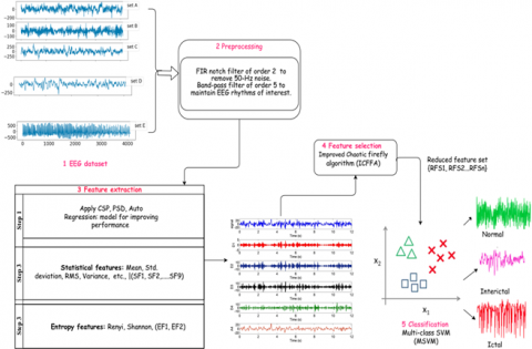
In this sub-section the proposed Epilepsy proposed epilepsy framework comprises of five phases such as dataset collection, signal pre-processing, feature extraction (FE), feature selection (FS) (i.e., optimization), and classification (see Figure 1). The first & second phases are the EEG dataset followed by the pre-processing phase with precise filtering strategies to remove artifacts. The third phase is a feature extraction of statistical features (SF1-SF9), entropy features (EF1-EF2) with the assistance of Power Spectral Density (PSD), Common spatial pattern (CSP), and Autoregressive (AR) model. The fourth phase CFFA performs the feature selection process that results in reduced feature subset (RFS1, RFS2, ..., RFSn) which can be used to build and test the multi-class SVM classifier (M-SVM) in the final phase.
3.1 EEG data selection
In this paper, we used the publicly available data set [16] that comprises of 5 sets, namely (A, B, C, D, and E), each with 23.6 seconds of EEG blocks with 100 individual channels. EEG recordings with severe artifacts like activity in eye muscles, and noise variations can be removed using Principal component analysis (PCA) with automatic target generation process (ATGP), and other artifact removal methods [17]. In this work, we are concerned with a three-class case that accompanies with the PSD, which provides us an energy distribution across frequency bins, whose frequency ranges differ and which can be very useful for extraction. The CSP procedure helps to separate the relevant and non-relevant channels from EEG signals (i.e. channel selection). Finally, the use of a prediction filter AR pattern improves EEG signal accuracy [18].
The first phase is the EEG dataset followed by the pre-processing phase with precise filtering strategies to remove artifacts. The third phase is a feature extraction of statistical features (SF1-SF9), entropy features (EF1-EF2) with the assistance of PSD, CSP, and AR model. The fourth phase CFFA performs the feature selection process that results in reduced feature subset (RFS1, RFS2, ..., RFSn) which can be used to build and test the multi-class SVM classifier in the final phase.
3.2 Preprocessing
The preprocessing phase is customized to suit all requirements of artifacts and noise removal to preserve the EEG rhythms. All the specifications are provided in the proposed diagram.
3.3 Feature extraction
It is the process of decreasing the amount of data (i.e., dimension) for obtaining less computation time for further process. The epileptic EEG varies considerably with the frequency, duration, intensity of the regular EEG signal, etc.
Feature vectors Extraction using DWT: Each EEG signal is decomposed by discrete wavelet transformation (DWT) into 5 constituent EEG sub-bands. We analysed the EEG epochs into different frequency bands using 4th-order wavelet feature Daubechies (db4) up to 4th level of decomposition as shown in Figure 2. The EEG signals were then decomposed into D1-D4 information and one final approximation of A4. For each EEG segment, the first, second, third, and fourth-level detail-wavelet coefficients (dk, k = 1, 2, 3, 4) in the order of (129 + 66 + 34 + 18 coefficients) and fourth-level approximation wavelet coefficients (a4) (18 coefficients) were determined. Thereafter, 265 wavelet coefficients for each EEG section were obtained. The wavelet coefficients of the EEG signals formed the first diverse feature vector representing the EEG signals.
Figure 1. Overview of proposed 5-phase framework
Figure 2. Arrangement of discrete wavelet transform (DWT)
In this paper, we have extracted the statistical values like Standard deviation (SD), Entropy, Variance, Median, Kurtosis, Skewness, Co-variance, Energy of wavelet coefficients from each sub-band that were chosen to classify EEG signals. By removing the data redundancy that has been stored in continuous wavelet transformation, DWT enables computation simpler and more efficient. To evaluate both frequency components, DWT of a signal s[n] is considered as it passes through a series of low pass filter (LPF) and high-pass filter (HPF).
$Ylow[n]=s[n]*g[n]=\sum\limits_{k=-\infty }^{\infty }{s[k]}.g[n-k]$ (1)
$Yhigh[n]=s[n]*h[n]=\sum\limits_{k=-\infty }^{\infty }{s[k]}.h[n-k]$ (2)
In Eqns. (1) and (2) the terms g[n] and h[n] indicate the impulse response of both filters (i.e. LPF and HPF). Although it undergoes down sampling the filter does not loss any information.
$Ydownsample[n]=\sum\limits_{k=-\infty }^{\infty }{s[k]}.g[2n-k]$ (3)
Shannon entropy method: This is the strongest lossless compression available, which provides low and high values of entropies that can be formulated asIn addition to boost the classifiers performance Shannon and Renyi entropies are used as parameters for classifier.
$E(S)=-q\sum\limits_{i=1}^{n}{pi\log 2pi,q=1}$ (4)
where, S signifies the EEG signal, pi the average probability and n the total number of EEG signal vector count.
Renyi entropy method: Renyi is the generalized from of Shannon entropy with α=1 and quadratic entropy with α=2, so their respective equation can be written as
$Eq(S)=\frac{1}{1-q}\log \sum\limits_{i=1}^{n}{\mathop{pi}^{q}}$ (5)
where, q≥0 and q≠1. Here, q in the Eq. (5) signifies the entropy order and variable n stand for total values of EEG data.
3.4 Feature selection
The primary goal of this work is to reduce the number of selected features and improve classification accuracy that can be treated to be multi-objective optimization problem. To take these two goals into consideration, so it can be formulated as a linear weighting solution to the fitness function as
$\Psi FS=x.E+y\frac{R}{C}$ (6)
and
$E=\frac{\text{ No}\text{. of wrongly predicted instance}}{\text{ Total number of instances}}$ (7)
In Eq. (7) E denotes the classification error, R denotes selected features from the subset C denotes total number of features available in the dataset. The weights used in comparisons x and y meet two of these objectives.
Firefly optimization Algorithm: The primary intention of the sub-section is twofold. First, to exemplify the improving firefly through the development of chaotic maps for chaotic FFA and second, to use logistic-tent maps (LTM) for faster convergence, and robustness to solve feature selection problem. According to Marie-Sainte' study [19] the flash frequency reduces as distance (r) rises with that of the equation
$I\left( r \right)={{I}_{0}}{{e}^{-\gamma {{r}^{2}}}}$ (8)
Attractiveness (β) is described in the map with an absorption coefficient (γ) and distance (r) as
$\beta \left( r \right)={{\beta }_{0}}{{e}^{-\gamma {{r}^{2}}}}$ (9)
The Cartesian distance between and two ith and jth fireflies at xi and xj respectively, the Cartesian distance is determined by
${{r}_{ij}}=\sqrt{\sum\limits_{k=1}^{d}{{{\left( {{x}_{i,k}}-{{x}_{j,k}} \right)}^{2}}}}$ (10)
where, xi,k is the kth element of the x of ith firefly d space coordinate, the number of dimensions is. The firefly movement happens if it is drawn to another (brighter) jth firefly that is defined by the equation.
${{x}_{i}}={{x}_{i}}+{{\beta }_{0}}{{e}^{-\gamma r_{ij}^{2}}}\left( {{x}_{j}}-{{x}_{i}} \right)+\alpha \in$ (11)
${{\beta }_{0}}{{e}^{-\gamma r_{ij}^{2}}}\left( {{x}_{j}}-{{x}_{i}} \right)$ is due to attraction.
α ϵ is due to randomization.
α is the randomization parameter.
ϵ is a vector of random numbers drawn from Gaussian or uniform distribution.
According to Gupta' study [20], the algorithm involves in decreasing the randomness gradually and incorporating the social dimension for every firefly (i.e., global best). The distance function (ri) put in the mathematical form as
${{r}_{i,best}}=\sqrt{{{\left( {{x}_{i}}-{{x}_{gbest}} \right)}^{2}}+{{\left( {{y}_{i}}-{{y}_{best}} \right)}^{2}}}$ (12)
The movement of ith firefly is determined by the equation
$x_{i}=x_{i}+\left(\beta_{0} e^{-\gamma r_{i, j}^{2}}\left(x_{j}-x_{i}\right)+\beta_{0} e^{-\gamma r_{i, \text { best }}^{2}}\left(x_{\text {gbest }}-x_{i}\right)\right)+\alpha \in+\lambda \in\left(x_{i}-g_{\text {best }}\right)$ (13)
Here ith because the firefly came up with the best solutions if there was no perfect local best solution in the neighborhood. This above algorithm thus decreases the algorithm randomness so that convergence is achieved rapidly and affects fireflies’ movement towards global optimal, thus decreasing the algorithm's probability caught in several local optima.
In Eq. (13) α is the randomization parameter and ∈ is the random number vector. Although the algorithm has no specific selection criterion, it changes each firefly in each iteration step and ranks it by fitness value and then selects individual potential. The classifier learning accuracy decides the fitness value and the firefly with the higher value that is known as a potential individual. The fitness function considered here for evaluating the feature sub-set is seen in the updated Eq. (13)
$\begin{align} & \mathop{Fitness}_{val}=\eta *\mathop{predictive}_{acc} \\ & +\left( 1-\eta \right)*\mathop{feature}_{redu} \\\end{align}$ (14)
In Eq. (14) η(1-η) and (1-η) are the parameters corresponding to weight of the learning accuracy.
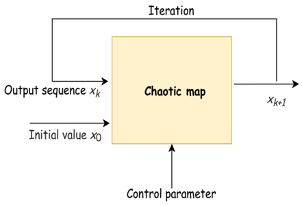
Chaotic Maps: Chaos is a stochastic movement defined by a deterministic equation which varies from the phenomena of irregularity and disorder. Chaos has a perfect internal structure. Random, ergodic and regular with three characters. Ergodic property can test all states in a certain range by its formulas. This has made chaos a technique accessible that keeps them from getting trapped in local optima and increases the search efficiency globally. In this paper, the firefly’s population is instantiated and we substitute the continuous absorption of the coefficient value with chaotic maps (see Figure 3).
Figure 3. Chaotic map processing
Three parameters regulate an initial feature, i.e. the random movement step size α, attractiveness β and absorption coefficient γ. In Eq. (14), the first parameter affects the randomized term α$\in $i, in which we set the randomized parameter $\in $i using chaos time series.
$\mathop{\in }_{i}=\mathop{C}_{i}^{(k)}$ (15)
Following chaotic-enhanced form,
$\mathop{\beta }_{i}=\mathop{\beta }_{0}\mathop{C}_{i}^{(k)}$ (16)
Remarkably, the firefly social factor of move can be specified by approximately overviews based on Yang' study [21]. The most commonly utilized chaotic activity is the logistic map and tent map. They are both close and exhibit chaotic dynamics. Chaotic sequences can rapidly and efficiently be produced and processed, without long sequence storage. In this paper, chaotic sequences incorporated in ICFFA is used to calculate the initial weight values where k shows the number of iterations and the logistic map and the tent map.
Logistic maps are expressed as
$\mathop{x}_{k+1}=\mathop{\mu x}_{k}\left( \mathop{1-x}_{k} \right)$ (17)
where, $\mu \in [0,4]$ and $x\in [0,1]$, xktakes any value from 0 to 1 belongs to the feature-extraction input value. k is the number of iterations; μ is the interval control parameter (1, 4) to decide how many maps numbers to complete the function collection are needed. A number sequence provided by the iteration of a logistic map (orbit also) with μ = 4 is chaotic. For values above 4 (μ > 4). The maps return negative values that reduce the efficiency of the algorithm.
Tent Map: It is an iterated method that shapes a discreet dynamic system is in the shape of a tent. It begins on the actual line from a point xk and maps it to a different end. It is an equation with a certain value of the control parameter (μ). With chaotic behavior, it is rather dynamic. It describes the map of the tent as
$x_{k}+1=\left\{\begin{array}{c}\mu x_{k} / 2, \text { for } x_{k}<0.5, \\ \mu\left(1-x_{k}\right) / 2, \text { for } x_{k} \geq 0.5\end{array}\right.$ (18)
where, μ is in the range [0, 2] and it is a positive real constant.
Tent map suffers from periodic window conflicts. Conversely, the classical chaotic systems such as the tent and logistic maps have certain inadequacies such as non-uniform data distribution. In the current article, we use Joint Logistic-Tent Map (JLTM) to ease periodic window issues. The multiple chaotic map shows a stable chaotic distribution between 0 and 4.
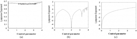
Similarly, Lyapunov’s exponent of multiple chaotic map like Logistic-Tent Maps (LTM) are seen in Figure 4(a) shows positive values that lies in the range of (0, 4), while in Figure 4(b) and Figure 4(c), Lyapunov’s one-dimensional map exponent has a set of non-positive values for logistic map (LM) and tent map (TM). So we used Logistic-Tent Maps (LTM) in the current paper to study.
Joint Logistic-Tent map (JLTM): It is multiple chaotic maps that can solve the problem of one-dimensional chaotic map can be inferred as stated earlier non-uniform distribution over output series that causes false selection in the features. To resolve we embed functions and weights to the model as (19a).
$x_{k+1}=G_{\mu}\left(x_{k}\right):$$=\left\{\begin{array}{l}\omega_{1} f_{1}^{\circ} F\left(\mu, x_{k}\right)+\alpha_{1} g_{1}\left(\mu x_{k}\right) \\ +\xi_{1} \frac{\left(\beta_{1}-\mu\right) x k}{2} \bmod 1, \text { when } x_{k}<0.5 \\ \omega_{2} f_{2}^{\circ} F\left(\mu, x_{k}\right)+\alpha_{2} g_{2}\left(\mu_{x k}\right) \\ +\xi_{2} \frac{\left(\beta_{1}-\mu\right)\left(1-x_{k}\right)}{2} \bmod 1, \text { when } x_{k} \geq 0.5\end{array}\right.$ (19a)
Figure 4. Lyapunov Exponent of multiple and Single Chaotic Map (a) Logistic-Tent map (LTM) (b) Logistic map (LM) (c) Tent map (TM)
where, F(μ, xk) is Logistic map. In (19a), fi(x) and gi(x) (i = 1, 2) for all the trigonometric functions. Correspondingly the terms, ωi, αi, ξi and βi (i = 1, 2) are real numbers and parameter μ $\in $ (0, 4]. For discrete time system (DTS) as (19a), the Lyapunov exponent for an orbit beginning with x0 is demarcated as
$LE(\mathop{x}_{0},\mu ):=\underset{n\to \infty }{\mathop \lim \frac{1}{n}}\,\sum\limits_{i=0}^{n-1}{\ln \left| \mathop{G}_{\mu }^{'}(\mathop{x}_{i}) \right|}$ (19b)
The degree of “sensitivity to initial conditions” measured with the help of the Lyapunov exponent. The pseudocode of a FFA with Joint Logistic-Tent map (ICFFA) for feature optimization (see Figure 5), the different parameter values for the ICFFA model (see Table 1).
Table 1. Parameter settings for the ICFFA model
|
Parameters |
Values |
|
Swarm size of ICFFA |
30 |
|
Number of generations for ICFFA |
500 |
|
Randomization |
0.6 |
|
Light absorption coefficient |
0.6 |
|
Attractiveness |
1 |
|
Chaotic parameter |
[1, 4] |
|
Chaotic map |
Logistic-Tent |
Figure 5. Pseudocode of an FFA with Joint Logistic-Tent map (ICFFA)
3.5 Classification
Several optimal feature subsets are supplied to the classifier to improve the performance. The viability of the framework is supported by comparison metrics with literature works. Taking advantage of extending binary classifier to multi-class classifier using SVM, we opted this for classification of EEG data. In this current study we dealt with three-class case, so the Multi-class SVM classifier is adopted by allocating code word with length N given as
$t(c)\in \mathop{\{-1,0,1\}}^{N}$ (20)
$t(c)\in \mathop{\{0,1\}}^{N},t(c)\in \mathop{\{-1,1\}}^{N}$ (21)
or for each class c. To eliminate over fitting problem in learning process some sort of slack terms is embedded with function f that can be written as
$Maximize\frac{\lambda }{M}\sum\limits_{m=1}^{M}{\mathop{\ell }_{m}}+\Omega \{f\}(m\arg in)$ (22)
To maintain the minimal distance between embedded function f, correct class target of interest t(y) and non-target of interest t(c). Then it can be generalized to optimized problem to the minimizing as
$Minimize\frac{\lambda }{M}\sum\limits_{m=1}^{M}{\mathop{\ell }_{m}}+\Omega \{f\}$ (23)
From the above analysis, it is explicitly that MSVM classifier optimal problem is w.r.t the soft margin and distance function d.
In this paper, we chose Matlab 2017b software for carrying simulation due to efficient toolboxes support for EEG signal analysis. The benchmark dataset used in this study is from Bonn University that contains 5 classes and 100 cases for each class. After artifact visual inspection, e.g. muscle activity or eye movements, these fragments were collected and segmented by continuous EEG multi-channel recordings. EEGs were selected for five patients, all of whom were correctly identified as an epileptogenic region following resection of any of the hippocampal structures.
Performance metrics: The performance metrics are conducted to show the effectiveness of the framework like Sen, Spec, Acc, etc.,
During the experiment, five separate statistical parameters were measured and evaluated per each run. It provides specifics of the following parameters:
Mean: It is the average of picking feature count form the total number of features taken after every iteration as
$Mean=\frac{1}{M}\sum\limits_{i=1}^{M}{size\left( \mathop{g}^{*i} \right)}$ (24)
where, g*i signifies optimal solution during the ithrun.
Best value: It is the process of getting the best (lowest) value among all the available fitness values that can be obtained throughout the iterations as
$\mathop{\min }_{1\le i\le M}\left( \mathop{g}^{*i} \right)$ (25)
Worst value: It is the process of getting the worst (highest) value among all the available fitness values obtained throughout the iterations as
$\mathop{\max }_{1\le i\le M}\left( \mathop{g}^{*i} \right)$ (26)
Standard Deviation: It is the process of showing the reflection for variance/dispersion for the central value of data series, i.e. the concentration or dispersion of the multiple outputs about the mean value. It can be formulated as follows:
$SD=\sqrt{\frac{1}{M-1}}\sum{\mathop{\left( \mathop{g}^{*i}-Mean \right)}^{2}}$ (27)
Analysis of Complexity after feature selection: The computation complexity of traditional firefly algorithm is (O (n2)) in which n signifies population and t iteration count. When n is large use it by taking the help of attractiveness β ranking with sorting mechanisms. Therefore, by global optimization mobility of chaotic firefly the complexity can be reduced to O(nt(log(n)). The computation complexity of statistical and entropy features is calculated and presented (see Table 2).
Table 2. Computation complexity of statistical and entropy features
|
Analysis |
Training time (in sec) |
Testing time (in sec) |
|
Statistical features + Multi-class SVM |
220 |
140 |
|
Statistical features + ICFFA+ Multi-class SVM |
203 |
130 |
|
Entropy features + MSVM |
240 |
160 |
|
Entropy features + ICFFA+MSVM |
212 |
142 |
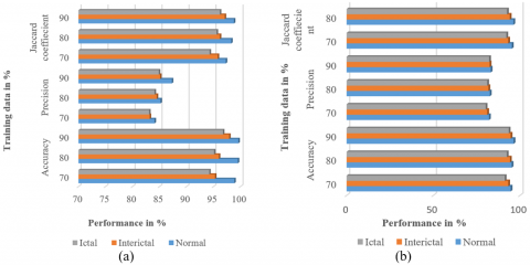
The training and testing time of classifier on y-axis and statistical, entropy features with and without feature selection process along with type of approach on x-axis (see Figure 6). It is clear that both the training and testing time of (statistical features + ICFFA + Multi class SVM, Entropy features + ICFFA+ MSVM) is less as compared to (statistical features + Multi class SVM, Entropy features + MSVM) because overfitting problem is eliminated on applying feature selection technique and good learning model capability (i.e., ICFFA). The performance metrics considered in this study for 70%, 80% and 90% training data in terms of Sen, Spec, Acc, Prec, Recall and JC with feature selection (FS) CFFA+ MSVM and without feature selection (FS) CFFA+ MSVM classifiers (see Tables 3-6). The average accuracy over three-class case with ICFFA+ MSVM classifier (see Figure 7(a)). It is evident from the figure; the accuracy is reached to 99.63%. Similarly, three-class case (i.e., AB-CD-E) which results in poor performance in terms of accuracy, precision and Jaccard coefficient, without feature selection, due to suffering from overfitting or inefficient learning model; due to absence of feature selection and direct applying to the classifier (see Figure 7(b)).
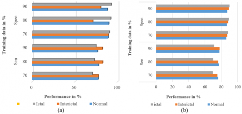
The better Sen, Spec values for three-class case with ICFFA+ MSVM classifier as compared to the MSVM classifier without ICFFA (see Figure 8(a)-(b)). The comparison of the works suggested in this paper (Average of three cases: Normal- Interictal-Ictal for 90% Training data). It shows that Chaotic FFA (ICFFA) +MSVM classifier outperforms as compared to its variants in three cases (i.e. Accuracy, Sensitivity and Jaccard coefficient). A bold font for a simple presentation illustrates the best values achieved from a specified method (see Table 7).
Figure 6. Comparison of training and testing time of statistical and Entropy features
Figure 7. Comparison of Acc, Prec and JC of three-class case (a) with ICFFA+ MSVM classifier (b) without ICFFA+ MSVM classifier
Table 3. Acc, Pre and JC with ICFFA+MSV
|
With FS |
Accuracy (Acc) |
Precision (Prec) |
Jaccard coefficient (JC) |
||||||
|
Training in (%) |
70 |
80 |
90 |
70 |
80 |
90 |
70 |
80 |
90 |
|
Normal |
98.88 |
99.53 |
99.63 |
84.1 |
85.2 |
87.3 |
97.3 |
98.3 |
98.8 |
|
Interictal |
95.3 |
96.01 |
97.92 |
83.2 |
84.5 |
85.13 |
95.8 |
96.2 |
97.1 |
|
Ictal |
94.23 |
95.12 |
96.77 |
83.1 |
84.1 |
84.89 |
94.3 |
95.6 |
96.2 |
Table 4. Sen, Spec and F-measure with ICFFA+MSVM
|
With FS |
Sen |
Spec |
F-measure |
||||||
|
Training in (%) |
70 |
80 |
90 |
70 |
80 |
90 |
70 |
80 |
90 |
|
Normal |
77.17 |
77.72 |
76.49 |
88.9 |
89.6 |
87.9 |
0.80 |
0.85 |
0.92 |
|
Interictal |
77.16 |
82.46 |
82.09 |
88.9 |
70.9 |
80.17 |
0.79 |
0.81 |
0.82 |
|
Ictal |
70.37 |
72.58 |
74.58 |
90.23 |
91.94 |
92.44 |
0.75 |
0.76 |
0.81 |
Table 5. Acc, Prec and JC with MSVM classifier
|
Without FS |
Accuracy(Acc) |
Precision (Prec) |
Jaccard coefficient (JC) |
||||||
|
Training in (%) |
70 |
80 |
90 |
70 |
80 |
90 |
70 |
80 |
90 |
|
Normal |
94.6 |
95.2 |
96.3 |
82.1 |
82.6 |
83.1 |
95.3 |
96.2 |
97.2 |
|
Interictal |
93.2 |
94.2 |
94.6 |
81.1 |
81.8 |
82.5 |
93.2 |
94.1 |
94.8 |
|
Ictal |
91.2 |
92.4 |
93.5 |
80.2 |
81.1 |
82.2 |
92.1 |
92.5 |
93.7 |
Table 6. Sen, Spec and F-measure with MSVM classifier
|
Without FS |
Sen |
Spec |
F-measure |
||||||
|
Training in (%) |
70 |
80 |
90 |
70 |
80 |
90 |
70 |
80 |
90 |
|
Normal |
76.2 |
77.1 |
77.8 |
86.2 |
86.8 |
87.2 |
0.75 |
0.81 |
0.89 |
|
Interictal |
75.2 |
76.2 |
77.9 |
87.2 |
88.5 |
89.3 |
0.74 |
0.75 |
0.78 |
|
Ictal |
69.5 |
70.1 |
71.2 |
88.2 |
89.2 |
90.1 |
0.73 |
0.74 |
0.75 |
Figure 8. Comparison of Sen, Spec of three-class case (a) with ICFFA+ MSVM classifier (b) without ICFFA+ MSVM classifier
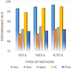
Table 7. Comparison of the average of three-class case: Normal-Interictal-Ictal for 90% Training data
|
Performance metric |
SFFA+ MSVM classifier [19] |
MFFA+ MSVM classifier [20] |
ICFFA + MSVM classifier |
|
Accuracy (Acc) |
96.23% |
97.11% |
98.11% |
|
Sensitivity (Sen) |
83.51% |
83.47% |
85.76% |
|
Specificity (Spec) |
85.84% |
87.23% |
86.84% |
|
Jaccard coefficient (JC) |
94.27% |
96.45% |
97.27% |
|
Precision (Prec) |
84.76% |
85.03% |
85.76% |
The three different methods of epilepsy detection for three-class case in which Improved Chaotic FFA (ICFFA) + MSVM classifier outperforms as compared to other two methods in terms of performance metrics (see Figure 9).
Assessment of Proposed ICFFA Algorithm: The overall performance of proposed ICFFA in terms of parameter tuning, we discuss statistical results. We know that a meta-heuristic algorithm is difficult to solve many optimization problems, particularly for identical parameter settings as per the No Free Lunch (NFL) principle. Therefore, important parameters are useful largely because it allows the optimization problem to be solved to get the best performance.
Figure 9. Comparison of different methods of detection of three-class case of epilepsy
Table 8. Parameter tuning results of c in ICFFA
|
Light absorption coefficient (c) |
Accuracy |
No. of Features |
Fitness value |
|
c=0.5 |
0.9830 |
8.26 |
0.0395 |
|
c=0.6 |
0.9963 |
6.25 |
0.0312 |
|
c=1 |
0.9897 |
9.66 |
0.0417 |
|
c=2 |
0.9812 |
10.43 |
0.0456 |
Table 9. Fitness values obtained by different chaotic maps in FFA
|
Chaotic map |
Best value |
Worst value |
SD |
Mean |
CPU time in (Sec) |
|
Logistic map |
0.0846 |
0.1241 |
0.0108 |
0.897 |
155.41 |
|
Tent map |
0.0763 |
0.1183 |
0.0101 |
0.835 |
148.32 |
|
Joint Logistic-Tent map |
0.0689 |
0.1012 |
0.0998 |
0.786 |
161.23 |
In addition, each combination runs for 30 times separately to eliminate arbitrary bias and it provides the cumulative results. We present the tuning effects of the parameter (see Table 8). Based on performance, ICFFA provides the best optimization results when it is c=0.6. Therefore, for all dataset instances, we use these parameter values. We have applied several statistical methods to better test the proposed ICFFA, and in this segment, it measures the fitness function values from different chaotic maps to explicitly demonstrate the efficiency of these approaches. The numerical statistical values for the best value, worst value, standard deviation (SD), we show average value and the CPU time of the various dataset approaches (see Table 9). A bold font for a simple presentation illustrates the best values achieved from a specified method.
This table displays the best performance of the Joint Logistic-Tent Map (JLTM) in contrast to other chaotic maps. In comparison, ICFFA requires more CPU usage on certain datasets to solve feature selection problems. This is because incorporated improved variables need additional solutions that increase the experimental time. The best performance of the Joint Logistic-Tent Map (JLTM) in contrast to other chaotic maps is achieved (see Figure 10). The comparison of the literature of results for 90% Training Data done by several authors are listed along with their overall accuracy and features used for EEG seizure detection (see Table 10).
From the Figure 11 it is evident that the Our proposed work shows superior performance when compared to literature of works due to adopting chaos which is best suitable for optimizing the output feature subset with less number of iterations and fast convergence.
Figure 10. Comparison graph of different chaotic maps in FFA
Table 10. Comparison of the literature of results for 90% training data
|
Author |
Features used |
Overall Accuracy in (%) |
|
Method 1 [22] |
Shannon Entropy+ GRNN, DT-CWT + Energy, STD |
97.21% |
|
Method 2 [23] |
PEN + SVM, DT-CWT + HE, FD |
98.22% |
|
Method 3 [24] |
DWT + Different Features + ANOVA-FSFS +LS-SVM |
99.50% |
|
Our work |
Statistical, entropy (Shannon and Renyi entropy) and DWT |
99.63% |
Figure 11. Comparison graph of overall accuracy for our work with traditional works
In this paper we proposed an integrated framework to Detect the epilepsy by proposing the framework of EEG signal exploration with the Multi-class SVM and Improved Chaotic Firefly algorithm (ICFFA). To accomplish the process of training/testing the classifier, this approach used the features obtained by statistical (DWT) and entropy-based examination for each subject of EEG data. After we built the feature set, a feature selection based on a chaotic mapping-based firefly version called ICFFA was used, which decreased the insignificant features to result in optimal feature subset. For obtaining this, two types of chaotic maps, a logistic map and a tent map, are used in combined form on FFA. However theses chaotic maps display different dynamic behavior between [0, 1]. The behavior affects the search ability of ICFFA. Then an MSVM classifier was trained with 70%, 80%, and 90% of data and tested with 30%, 20%, and 10% of the data, respectively. The Experimental results shows that the proposed technique (ICFFA+MSVM) attained a satisfactory accuracy of 99.63% for Normal data (Set A and B) and an accuracy of 98.10%, 97.3% of the JC, and 85.77% of precision (averaged for Normal, Inter-ictal and Ictal classes of data with 90% training). Also experimental results show that ICFFA with joint Logistic-tent map obtained higher success rate than CFFA alone with a logistic OR Tent map alone.
The authors wish to thank Andrzejak et al., 2001 for the benchmark EEG dataset available: http://www.meb.unibonn.de/epileptologie/science/physic/eegdata.html.
[1] Acharya, U.R., Sree, S.V., Swapna, G., Martis, R.J., Suri, J.S. (2013). Automated EEG analysis of epilepsy: A review. Knowledge-Based Systems, 45: 147-165. https://doi.org/10.1016/j.knosys.2013.02.014
[2] Fisher, R.S., Boas, W.V.E., Blume, W., Elger, C., Genton, P., Lee, P., Engel Jr, J. (2005). Epileptic seizures and epilepsy: Definitions proposed by the International League Against Epilepsy (ILAE) and the International Bureau for Epilepsy (IBE). Epilepsia, 46(4): 470-472. https://doi.org/10.1111/j.0013-9580.2005.66104.x
[3] Ji, Z., Sugi, T., Goto, S., Wang, X., Ikeda, A., Nagamine, T., Shibasaki, H., Nakamura, M. (2011). An automatic spike detection system based on elimination of false positives using the large-area context in the scalp EEG. IEEE Transactions on Biomedical Engineering, 58(9): 2478-2488. https://doi.org/10.1109/TBME.2011.2157917
[4] Xia, Y., Leung, H. (2006). Nonlinear spatial-temporal prediction based on optimal fusion. IEEE Trans. Neural Networks, 17(4): 975-988. https://doi.org/10.1109/tnn.2006.875985
[5] Al-Tashi, Q., Rais, H., Jadid, S. (2018). Feature selection method based on grey wolf optimization for coronary artery disease classification. International Conference of Reliable Information and Communication Technology, Kuala Lumpur, Malaysia, pp. 257-266. https://doi.org/10.1007/978-3-319-99007-1_25
[6] Mafarja, M., Mirjalili, S. (2018). Whale optimization approaches for wrapper feature selection. Applied Soft Computing, 62: 441-453. https://doi.org/10.1016/j.asoc.2017.11.006
[7] Arora, S., Anand, P. (2019). Binary butterfly optimization approaches for feature selection. Expert Systems with Applications, 116: 147-160. https://doi.org/10.1016/j.eswa.2018.08.051
[8] Adamczyk, M. (2014). Parallel feature selection algorithm based on rough sets and particle swarm optimization. 2014 Federated Conference on Computer Science and Information Systems, Warsaw, Poland, pp. 43-50. https://doi.org/10.15439/2014F389
[9] Shokouhifar, M. (2011). An ant colony optimization algorithm for effective feature selection. Proc. 3rd International Conference on Machine Learning and Computing (ICMLC), pp. 36-40.
[10] Yang, X.S. (2009). Firefly algorithms for multimodal optimization. International Symposium on Stochastic Algorithms, Sapporo, Japan, pp. 169-178. https://doi.org/10.1007/978-3-642-04944-6_14
[11] Slimen, I.B., Boubchir, L., Mbarki, Z., Seddik, H. (2020). EEG epileptic seizure detection and classification based on dual-tree complex wavelet transform and machine learning algorithms. Journal of Biomedical Research, 34(3): 151-161. https://doi.org/10.7555/JBR.34.20190026
[12] Agboola, H., Solebo, C., Aribike, D., Lesi, A., Susu, A. (2019). Seizure prediction with adaptive feature representation learning. Journal of Neurology and Neuroscience, 10(2): 294. https://doi.org/10.36648/2171-6625.10.2.294
[13] Pramudita, B.A., Wibirama, S., Izhar, L.I., Setiawan, N.A. (2018). EEG Motor imagery signal classification using firefly support vector machine. 2018 International Conference on Intelligent and Advanced System (ICIAS), Kuala Lumpur, pp. 1-6. https://doi.org/10.1109/ICIAS.2018.8540578
[14] Anter, A.M., Wei, Y., Su, J., Yuan, Y., Lei, B., Duan, G., Mai, W., Nong, X., Yu, B., Li, C., Fu, Z., Zhao, L., Deng, D., Zhang, Z. (2019). A robust swarm intelligence-based feature selection model for neuro-fuzzy recognition of mild cognitive impairment from resting-state fMRI. Information Sciences, 503: 670-687. https://doi.org/10.1016/j.ins.2019.07.026
[15] Abdel-Basset, M., El-Shahat, D., El-henawy, I., de Albuquerque, V.H.C., Mirjalili, S. (2020). A new fusion of grey wolf optimizer algorithm with a two-phase mutation for feature selection. Expert Systems with Applications, 139: 112824. https://doi.org/10.1016/j.eswa.2019.112824
[16] Abbasi, R., Esmaeilpour, M. (2017). Selecting statistical characteristics of brain signals to detect epileptic seizures using discrete wavelet transform and perceptron neural network. International Journal of Interactive Multimedia & Artificial Intelligence, 4(5): 33-38.
[17] Vijaykumar, J., Srinivasa Reddy, E. (2019). A robust system for detection of artifacts from EEG brain recordings. International Journal of Innovative Technology and Exploring Engineering, 9(2): 3947-3951. https://doi.org/10.35940/ijitee.B6909.129219
[18] Vijaykumar, J., Srinivasa Reddy, E., Elemo, T.K. (2020). Epileptic seizure prediction based on features extracted using wavelet decomposition and linear prediction filter. International Journal of Scientific & Technology Research, 9(2).
[19] Marie-Sainte, S.L., Alalyani, N. (2020). Firefly algorithm based feature selection for Arabic text classification. Journal of King Saud University-Computer and Information Sciences, 32(3): 320-328. https://doi.org/10.1016/j.jksuci.2018.06.004
[20] Gupta, D., Gupta, M. (2016). A new modified firefly algorithm. International Journal of Recent Contributions from Engineering, Science & IT (iJES), 4(2): 18-23. http://dx.doi.org/10.3991/ijes.v4i2.5879
[21] Yang, X.S. (2010). Firefly algorithm, Levy flights and global optimization. In: Bramer M., Ellis R., Petridis M. (eds) Research and Development in Intelligent Systems XXVI. Springer, London. https://doi.org/10.1007/978-1-84882-983-1_15
[22] Swami, P., Gandhi, T.K., Panigrahi, B.K., Tripathi, M., Anand, S. (2016). A novel robust diagnostic model to detect seizures in electroencephalography. Expert Systems with Applications, 56: 116-130. https://doi.org/10.1016/j.eswa.2016.02.040
[23] Li, M., Chen, W., Zhang, T. (2017). Automatic epileptic EEG detection using DT-CWT-based non-linear features. Biomedical Signal Processing and Control, 34: 114-125. https://doi.org/10.1016/j.bspc.2017.01.010
[24] Chen, S., Zhang, X., Chen, L., Yang, Z. (2019). Automatic diagnosis of epileptic seizure in electroencephalography signals using nonlinear dynamics features. IEEE Access, 7: 61046-61056. https://doi.org/10.1109/ACCESS.2019.2915610