Di Wu | Chunjiong Zhang* | Li Ji | Rong Ran | Huaiyu Wu | Yanmin Xu
© 2021 IIETA. This article is published by IIETA and is licensed under the CC BY 4.0 license (http://creativecommons.org/licenses/by/4.0/).
OPEN ACCESS
Forest fire recognition is important to the protection of forest resources. To effectively monitor forest fires, it is necessary to deploy multiple monitors from different angles. However, most of the traditional recognition models can only recognize single-source images. The neglection of multi-view images leads to a high false positive/negative rate. To improve the accuracy of forest fire recognition, this paper proposes a graph neural network (GNN) model based on the feature similarity of multi-view images. Specifically, the correlations (nodes) between multi-view images and library images were established to convert the input features of graph nodes into the correlation features between different images. Based on feature relationships, the image features in the library were updated to estimate the node similarity in the GNN model, improving the image recognition rate of our model. Furthermore, a fire area feature extraction method was designed based on image segmentation, aiming to simplify the complex preprocessing of images, and effectively extract the key features from images. By setting the threshold in the hue-saturation-value (HSV) color space, the fire area was extracted from the images, and the dynamic features were extracted from the continuous frames of the fire area. Experimental results show that our method recognized forest fires more effectively than the baselines, improving the recognition accuracy by 4%. In addition, the multi-source forest fire data experiment also confirms that our method could adapt to different forest fire scenes, and boast a strong generalization ability and anti-interference ability.
forest fire recognition, multi-view images, graph neural network (GNN), convolutional neural network (CNN), feature extraction
Forest fires pose a serious threat to the ecosystem of forests. To prevent the spread and hazards of the fire, the key lies in early detection of the fire source before the fire evolves into a catastrophe [1]. With the rapid development of computer vision, forest fire monitoring based on computer vision has become a hot topic among researchers of forest fire prevention. Color recognition is one of the earliest approaches for fire recognition. This approach recognizes the flame based on the movement, space, and time features of the color mode [2]. But color recognition can only identify large flames in a short distance. In recent years, convolutional neural network (CNN) has been introduced to forest fire recognition. For example, Khan Muhammad identified fire areas with a deep CNN, which avoids the tedious and time-consuming extraction of features, and automatically learns the rich features in the original fire data [3]. Despite its high recognition accuracy, the CNN only applies to the recognition of static fire images [4]. Saulskii et al. [5] attempted to automatically extract and classify fire image features with a deep normalized CNN (DNCNN). Noureddine et al. [6] proposed a detection framework based on Faster three-dimensional CNN (3DCNN) and faster region-based CNN (Faster RCNN). These networks face a high application cost, due to their huge computing load. Later, Emmy Prema adopts the background difference method to find moving pixels, and looks for flame color regions with a color model; Afterwards, a spatiotemporal analysis was performed on these regions to identify irregular and flickering fire features [7].
The above studies have only analyzed single-view images. In reality, forest fires cannot be monitored effectively without multiple monitors deployed in different perspectives. The single-view images cannot fully characterize the entire appearance of monitoring points. Therefore, it is not ideal to recognize fires based on single-view images [8]. However, the images on the same forest fire scene must be recognized first, in order to analyze the information of images with different views. In the same forest fire scene, the images taken from different angles usually carry the same fire features, namely, fire area, background color, and thermal radiation. Based on these features, researchers have designed various metrics for the similarity between multi-view images [9]. But these metrics emphasize the global similarity over the local similarity between two images. Take the measurement of the similarity between detection image and target image for example. In most cases, feature learning and metric learning merely test the pair relationship between single images, failing to consider the other relationships between images from different sources (e.g., the same image background, and similar items in the images). To overcome the problem, it is necessary to find the differences between images that reflect image features. Through manifold learning, Cao et al. [9] mapped images into manifolds, such that the local geometries of images are smoother for the analysis of image similarity. Kaliyamurthi et al. [10] relied on the similarity between re-sorted images to estimate the local similarity between images. However, manifold learning and re-sorting are mostly unsupervised, and their effects cannot be evaluated easily.
In recent years, graph neural network (GNN) has attracted much attention for its strong ability to generalize image data [11]. The GNN transmits information in a graphic structure, derives the final representation of each node through graph decomposition, and classifies the nodes. In the GNN, each image is entirely represented as graph nodes. Compared with manifold learning and re-sorting, the GNN enhances the end-to-end property of training, and facilitates the learning of feature representations. The network combines graph computing with deep learning (DL) into a DL framework robust in similarity estimation and identification.
For the above reasons, this paper adopts the GNN model to recognize forest fires with multi-view images. Firstly, a small batch of multi-view images was paired with library images through supervised learning of initial visual features. Next, each pair of images was treated as a node on the graph, and used to generate the similarity between images. After that, the image information of model learning was transmitted between nodes to update and optimize the pair relationship associated with each node. On this basis, feature fusion weights were adopted for image recognition, producing the robust similarity estimates of multi-view images.
The main contributions of this research are as follows:
(1) A GNN of multi-view image similarity (MV_GNN) was proposed, which derives a node graph from multi-view images to represent the correlations between images, and estimates image similarity based on the feature relationship of the updated nodes. The proposed MV_GNN fully considers the information from multi-view images, and thus improves the recognition rate of forest fires.
(2) A fire area feature extraction method was presented to simplify the complex image preprocessing and effectively extract the key features from the images. The extracted features were imported to our model to increase the recognition accuracy of forest fires.
(3) Experiments on different fire datasets show that the proposed method can effectively recognize forest fires in different scenes, and boasts a strong application potential and anti-interference ability.
Some forest fire recognition algorithms are implemented based on physical technologies. They recognize forest fires based on the flame features like color, texture, and movement. Barmpoutis et al. [12] identified the dynamic behaviors and irregularities of fires in red-green-blue (RGB) and hue-saturation-intensity (HIS) color spaces. Arrue et al. [13] designed classification rules according to the separation between color component and brightness in light intensity-blue/green intensity-red/green intensity (YCbCr) color space. Sudhakar et al. [14] studied flame shape and rigid object movement, intelligently extracted features by optical flow information and flame behaviors, and thereby differentiated between different flames. Jilbab et al. [15] combined shape, color, and movement attributes into a multi-expert system framework for real-time flame recognition. Qin et al. [16] experimentally discovered that the flame has a low chromaticity in the HSV color space. Based on RGB color model, Kingma et al. [17] extracted pixel points from the flame, and recognized flames according to their growth and unordered features. Jeong et al. [18] quickly estimated the movement direction of fires, superimposed the direction on time, and recognized fires by the spread feature.
Thanks to the continuous development of DL, computer vision offers new insights to fire recognition. For instance, Sun et al. [19] developed a CNN for forest fire recognition, augmented the limited training samples by randomly initializing parameters, and achieved a good effect in fire classification. Heyns et al. [20] integrated traditional recognition method with neural network: AdaBoost and local binary pattern (LBP) were employed to initially recognize the images and extract the candidate regions for flames; Then, the features were extracted from the candidate regions and classified by the CNN. Attri et al. [21] applied the deep belief network (DBN) to recognize flames. Considering the volume difference between fire images and normal images, Cuomo et al. [22] trained residual network (ResNet) [23] with biased data, and recognized flames with the trained network. Alkhatib et al. [24] introduce a multi-layer denoising and automatic encoding network algorithm, and applied the algorithm to dozens of scenarios, including forest fire. Wang et al. [25] proposed a cascaded CNN algorithm, which identifies the static and dynamic flame features with two independent CNNs, respectively, and judged whether an image area is flame combining the results of the two networks [26]. Rahim et al. [27] designed a DNCNN for fire image recognition, and compared it with VGGNet and ZFNet. All three network models can accurately recognize single-view images, but perform poorly on multi-source samples. To solve the problem, Fu et al. [28] introduced the GNN to improve image recognition, using the relationships between images. Mukherjee et al. [29] proposed a graph-based scheme involving Laplacian spectrum and spatial structure. The scheme extends the properties of the convolutional filter to general graphs, and identifies disasters with the spatial structure of graphs.
Most existing GNNs have an inherent network structure, without considering the similarity of data distribution, i.e., the correlations between data. Unlike most GNNs, the proposed MV_GNN can generate more accurate feature fusion weights through the transmission of graph information, and thus effectively recognize forest fire images with multiple views.
To effectively the extract feature from multi-view images, this paper preprocesses the images in three steps: image segmentation, fire feature extraction, and dynamic feature extraction. Image segmentation cuts out the fire area from each image, reducing the background interference; Fire feature extraction helps to judge some fire behaviors; Dynamic feature extraction enables the prediction of fire occurrence based on the spread features.
3.1 Image segmentation
HSV color space describes colors more intuitively than RGB color space. The three components, namely, hue, saturation, and value, are closely associated with the color perception method of neural network [30]. The HSV color space can be defined as:
$V=\{x\left| x(H)\in [0,359] \right., x(S)\in [0,255], x(V)\in [0,255]\}$ (1)
where, x is a pixel in the HSV color space; x(h), x(s) and x(v) are the H, S, and V components of x, respectively. Hence, the fire color distribution can be obtained from the sample images containing forest fire areas. Figure 1 shows the three component values of pixels derived from the sample colors. Then, the fire shape was represented by the Gaussian mixed model. The pixels of the colors in the range of the distribution model were taken as the fire pixels.
Figure 1. H, S, and V components
To further reduce the amount of calculation, three two-dimensional (2D) projection planes were adopted to replace the three-dimensional (3D) distribution model. That is, the fire colors of the sample images were projected to the HS plane, HV plane, and SV plane. In each plane, the range of color distribution can be easily represented by one or two rectangles. Thus, it is possible to define a relatively simple 2D color distribution.
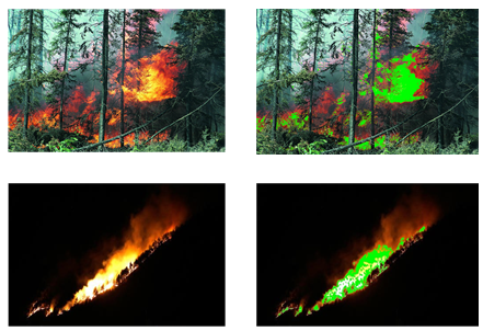
Based on color range, the images were segmented to identify the candidate fire areas. As shown in Figure 2, the forest fire scene was cut out (green area in the right subgraph) clearly.
Figure 2. Color-based fire area segmentation
3.2 Fire feature extraction
This step aims to acquire the size, roundness, and contour of each segmented fire area. Forest fires are initially unstable flames. Since fire pixels increases with fire area, size is an important feature of fire [7, 18]. To recognize the variability of fire area, the size change of fire area was calculated based on two consecutive images. Any size change surpassing the predefined threshold means the fire grows. The threshold could be the boundary chain code, roundness, and contour line of the fire.
For a given segmented fire area, the connected boundary chain code could be obtained easily by searching for the boundary of the area with the Laplacian operator. On this basis, the boundary circumference L could be calculated at ease. Then, the roundness of the fire area can be derived from L and the size of the fire area [25]. This parameter indicates the complexity of fire area shape. The more complex the shape, the greater the roundness. In early fire recognition, roundness helps to eliminate the interference by irregular bright objects.
The shape of the fire area changes due to the air flow. Thus, the degree of fire can be measured by the fluctuations of the contour. Suppose there are N points on the boundary, which can be described as complex numbers $\{{{z}_{i}}\left| {{z}_{i}}={{x}_{i}}+j{{y}_{i}} \right.\}$, where $\left( {{z}_{i}},{{y}_{i}} \right)$ is the coordinates of the i-th point on the fire area boundary in the clockwise direction. Then, the discrete Fourier transform of ${{z}_{i}}$ can be obtained:
${{F}_{w}}=\frac{1}{N}\sum\limits_{i=1}^{N}{{{z}_{i}}\exp (-j\frac{2\pi }{N}iw)} $ (2)
where, $F$ is the center of gravity of the one-dimensional (1D) boundary. Contour description is only needed for a few dozens of Fourier coefficients [4, 9, 16]. The first 32 $D=\left( {{\left| {{F}_{1}} \right|}_{2}},{{\left| {{F}_{2}} \right|}_{2}},\cdots ,{{\left| {{F}_{32}} \right|}_{2}} \right)$ were selected empirically. Then, the difference between two adjacent Fourier coefficients can be obtained as:
${{F}_{w}}=\frac{1}{N}\sum\limits_{i=1}^{N}{{{z}_{i}}\exp (-j\frac{2\pi }{N}iw)} $ (3)
If Ti is greater than the time threshold Td, and lasts longer than Tm, then the fire area shape has changed violently, indicating the possible occurrence of a fire. Td and Tm are thresholds obtained from test statistics.
3.3 Dynamic feature extraction
As the forest fire spreads, continuous fire images will carry the dynamic features of the fire. This is of great significance for fire detection [26]. This paper defines a dynamic feature containing n continuous images. The value of n should be a relatively small number to ensure the real-time detection of fires. In general, the flame flickers at a feature frequency of 10Hz, while the videos are recorded at 30 frames per second (fps) [22]. According to the needs of the real scene, the n value was set to 5, that is, the dynamic feature reflects the fire features of five continuous images. For the flame features in the images, an n´m matrix was constructed, where n=5 is the number of continuous images, and m=3 is the number of flame features, including size, roundness, and contour [12]. Suppose X(i,j) is an element corresponding to the i-th image and j-th flame feature. Then, the dynamic feature based on that matrix can be described by mean and mean squared error (MSE) [21]:
$E(j)=\frac{1}{n}\sum\limits_{i=1}^{n}{X(i, j)}$ (4)
$S(j)=\sqrt{\frac{1}{n}\sum\limits_{i=1}^{n}{{{\left( X(i, j)-E\left( j \right) \right)}^{2}}}}$ (5)
Therefore, any forest fire image has a dynamic feature, i.e., the mean and MSE of the image matrix. Our machine learning model was trained on forest fire images, supplemented by the information segmented from the images, fire features, and dynamic feature of the fire.
To evaluate our forest fire recognition algorithm, the test dataset was defined as the combination of a detection set and a library image set. The former tests the model performance, and the latter verifies the similarity between images in different fields. After being given a pair of detection images and multi-view images of the same scene, the forest fire recognition model aims to robustly determine the visual similarity between detection images. Our model was trained by a small batch of images. During the training, different image pairs were evaluated one by one, i.e., the similarity between images was measured one pair after another. In this way, the evaluation of one pair is not affected by other image pairs. Figure 3 explains the structure of the proposed MV_GNN model. A graph was generated from the inputs of a detection image and multiple library images. Each node models a pair of library images. The model outputs the similarity score of each library image. Through the end-to-end training, the deeply learned information was transmitted between the nodes, and used to update the relationships associated with each node, making similarity estimation more accurate.
Figure 3. MV_GNN
4.1 Graph representation and node features
In the proposed GNN model, each node represents a pair of library images. For a given library and n forest fire images, a complete undirected graph G(V, E) can be constructed, where V={v1, v2,…, vn} is the node set, and E is the edges between the nodes.
Firstly, the similarity score of each library image was evaluated. For any node, the complex relationship between the corresponding library images is encoded by the input feature. Figure 3(a) shows the input relationship feature obtained by our scheme. For a given library image and n forest fire images, each input image was imported to the share modular to encode the pair relationship feature.
The structure of the proposed share modular model is illustrated in Figure 3(a). The idea of ResNet [23] was adopted to prevent vanishing gradients, and share the CNN of network flow Scl and the parameters of fully connected layers (FCs) with the subsequent network layers, e.g., the edge for Scl and FC in Figure 2. This configuration enhances the soft mask of the information of network flow model, such that the model is more complete, accurate, and suitable for forest fire image recognition. The aim of Scl is to find the area that facilitates the target recognition in forest fire images. The CNN of the network flow involves classic optimization techniques like pooling layer, dropout, etc. Three FCs are right behind the CNN. The parameters of the FCs were shared with the subsequent network layers, and associated with the loss function.
Soft mask function was designed to reflect the importance of different model parameters [5, 24]. The function manifests the area in support of network prediction in the imported multi-view images, and enables the attention operation on the task of interest in the training network. Then, the information of forest fire images recognized by the network model is exactly what the model is expected to focus on (e.g., the specific forest fire color of the target). For this purpose, the soft mask of the network is trained from end to end, using the novel Mish activation function [25].
The last global mean set features of the two images in share modular were subtracted against each other to obtain pair relationship feature. These features were processed into differential features ${{d}_{i}}(i=1,2,\cdots ,n)$, i.e., the deep visual relationship between library images and the i-th image. The differential features were inputted to node i on the graph. The task on the graph is to classify the nodes, i.e., import the input features of each node into the linear classifier to output the similarity score, without considering the pair relationship between nodes. The loss function of our model takes the form of cross entropy:
$L=-\sum\limits_{i=1}^{n}{{{y}_{i}}\log (f({{d}_{i}}))+(1-{{y}_{i}})\log (1-f({{d}_{i}}))}$ (6)
where, f(×) is the sigmoid function of the classifier [27]; yi is the label of the i-th library image pair; l means the detection image has the same label as the i-th library image.
Besides measuring the similarity between a pair of detection images, the basic model in Figure 3(a) can calculate the similarity between detection image pairs. This facilitates the transmission of deep information, and the update of the relationship feature between detection image pairs. To transfer information more effectively, the image relationship feature di was imported to a two-layer message network for feature encoding (Figure 3(b)). Then, the similarity scores of the library were fused with the relationship feature of the library into a message transmission and feature fusion scheme.
4.2 Similarity guidance
This paper designs a similarity guidance scheme to help our model make full use of the similarity between different fields. The simple node classification model (6) ignores the valuable information between library pairs. To utilize this important information, an edge E was added on the fully-connected graph G. The edge E stands for the set of the relationships between library pairs. The scalar edge weight Wij, i.e., the importance of the relationship between nodes i and j:
${{W}_{ij}}=\left\{ \begin{align} & \frac{\exp (S({{g}_{i}},{{g}_{j}}))}{\sum\limits_{j}{\exp (S({{g}_{i}}, {{g}_{j}}))}}, i\ne j \\ & 0, i=j \\ \end{align} \right.$ (7)
where, gi and gj are the i-th and j-th images, respectively; S(gi, gj) is the similarity estimation function for a pair of images. The function estimates the similarity score between gi and gj , and establishes a model in a way similar to the node classification model.
To enhance the pair relationship feature between nodes, the deeply learned message was transmitted through all connected nodes. Then, the node features were updated into the weighted summation of all input messages and the original node features. Before the message transmission, each node must encode the deep message, so that it can be transmitted to the connected nodes. The input relationship feature di of each node was imported to a message network, which consists of two FCs, namely, Bayesian network (BN), and rectified linear unit (ReLU) [28]. The network would generate a deep message ti (Figure 3(b)). This process learning is suitable for the update of node relationship feature.
$t_{i}=F\left(d_{i}\right)$ for $i=1,2, \cdots, N$ (8)
where, $F(\cdot)$ is the two-layer FC network for deep message transmission. After the edge weight Wij and deep message ti of each node have been obtained, the node relationship feature di can be updated by:
${{d}_{i}}^{(1)}=(1-\alpha ) {{d}_{i}}^{(0)}+\alpha \sum\limits_{j=1}^{N}{{{W}_{ij}} {{t}_{j}}^{(0)}} \, for \, i=1,2,\cdots , N$ (9)
where, d(1) i is the relationship feature of the i-th image; d(0) i is the i-th input relationship feature; t(0) j is the deep message from node j; a is a weighted parameter to balance fused feature and original feature. The weighted fusion of relationship feature can be implemented iteratively:
${{d}_{i}}^{(k)}=(1-\alpha ) {{d}_{i}}^{(k-1)}+\alpha \sum\limits_{j=1}^{N}{{{W}_{ij}} {{t}_{j}}^{(k-1)}} \, for \, i=1,2,\cdots , N$ (10)
where, k is the number of iterations. The refined relationship feature d(k) i can replace the relationship feature di in formula (8) for loss function calculation and GNN training. During the training, formula (10) can update the framework and model through error backpropagation [24].
There are only a few low-resolution opensource image datasets about forest fire recognition. The authors collected and labeled lots of forest fire videos, and prepared a forest fire dataset based on the labeled videos. The dataset was uploaded to the opensource website (https://github.com/chunjiongzhang/fire-data). The fire dataset was formulated by crawling online forest fire images, segmenting the fire areas, and saving the segmented parts.
5.1 Techniques
Crawler is a technology that automatically collects the required information or resources online. This paper selects Python crawlers like Requests and Beautiful Soup [17]. OpenCV [31] is a cross-platform computer vision and image processing library. The Python interface of OpenCV was adopted for this research. Specifically, Cascade and Classifier are the cascading classifier of OpenCV for target recognition. The classifier uses the LBP to import the specific classifier files, e.g., image classifier, to realize the identification of targets [23].
5.2 Specific implementation
The preparation of forest fire image dataset must reduce the difficulty of manual check, in addition to ensuring quality and speed. In other words, the result of the program processing can only contain a very small number of non-fire images. Thus, this paper designs a screen module.
Single-threaded data writing, data analysis, and waiting for server response consume too much time, making it impossible to fully utilize the bandwidth. Therefore, the selected crawlers operated in a multi-threaded manner. The crawling speed depends on the upper limit of the bandwidth.
All the fire images acquired by the crawlers were processed by the cascade classifier of OpenCV. The saved fire images were subjected to local recognition, and the fire areas were segmented from the images. OpenCV alone cannot accurately recognize fire images. If there are sufficient original images, lots of non-fire images would be generated. Hence, the unqualified images were filtered out by the Dlib module.
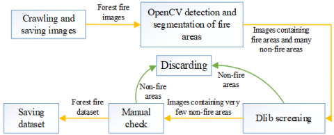
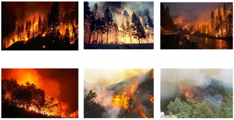
As shown in Figure 4, the dataset was prepared in three steps: collecting images with crawlers; cropping the fire areas in fire recognition module; filtering out the unqualified images in Dlib module. Figure 5 shows the contents of the prepared dataset.
Figure 4. Preparation of forest fire dataset
Figure 5. Contents of forest fire dataset
6.1 Dataset
The forest fire images were collected online with the technique proposed in Section 5. A total of 2,826 forest fire images were collected, including the images on fire outbreak and the images on fire spread. Meanwhile, 932 non-forest fire images were collected. All these images were collectively referred to as the forest fire dataset.
xBD dataset [32] is one of the public datasets of high-resolution labeled satellite images. The dataset on natural disaster images is updated by the Massachusetts Institute of Technology (MIT). It covers 22,068 images of 19 different disasters. The image resolution is 1,024×1,024. Every building in the dataset has an identifier. This paper only uses the images containing forest fires in xBD dataset.
6.2 Setup
Our model was realized under the framework of Keras and TensorFlow. The operation system is Ubuntu19.04; the graphics processing unit (GPU) is GeForce GTX 1080Ti; the central processing unit (CPU) is Intel Core i710500U with a RAM of 16GB and a hard disk of 1TB. Our model was compared with DL models like ResNet and DenseNet [28], using the learning rate of 0.01 and batch size of 64.
The proposed GNN recognizes forest fires based on the designed share modular. All input images were adjusted to the size of 256×128. Firstly, the basic CNN model was pretrained with the initial learning rate of 0.01 on all datasets. After 50 epochs, the learning rate was reduced by 10 times, and then maintained for 50 epochs. The weight of the linear classifier trained during the basic model training was adopted to initialize the weight of the linear classifier for image similarity measurement. The model was optimized by Adam [23], with the weighted parameter is 0.9.
6.3 Results
Table 1 records the number of parameters, training times, and test results of different models.
Table 1. Test results of different models
|
|
Model |
N* |
P* |
T |
A |
|
xBD Datase |
ResNet |
50 |
23,602,904 |
724.94 |
94.33 |
|
DenseNet |
50 |
1,477,058 |
1,153.9 |
96.15 |
|
|
MV_GNN |
50 |
768626 |
867.8 |
98.33 |
|
|
Forest fire dataset |
ResNet |
50 |
21,702,355 |
701.35 |
95.67 |
|
DenseNet |
50 |
1,142,587 |
1,023.44 |
97.85 |
|
|
MV_GNN |
50 |
548,633 |
804.83 |
99.02 |
Notes: N* is the number of layers, P* is total parameters, T is training time/s A is accuracy/%.
As shown in Table 1, our GNN model consumed a much shorter training time on the two datasets than DenseNet. The model can effectively utilize images of multiple views or sources, and converge quickly through data accumulation. Meanwhile, our model consumed comparable training time as ResNet, but with much fewer parameters. Besides, our GNN surpassed ResNet by 4% in accuracy. This is because our model extracts the dynamic feature of forest fire images in advance, and thus quickly learns the deep information of the images. Besides, our model has similarity guidance on forest fire images of multiple views or sources. In addition, our framework boasts the fewest parameters, which reduces the memory overhead. Overall, our model achieved good accuracies on different training sets, without producing overfitting. The results show that our scheme has a strong generalization ability, and a good robustness. Capable of identifying forest fire images of different views, our approach can satisfy the forest fire monitoring needs in different scenes.
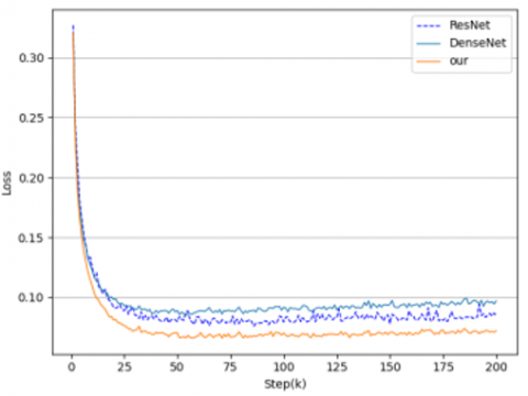
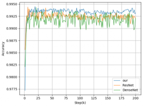
Figure 6. Loss and accuracy of model training
The loss decline in the left subgraph of Figure 6 indicates that our method converged faster than the baselines during xBD training, and remained stable throughout the training. Our model was completely trained in 27k epochs, while the latest DenseNet was not fully trained until the 32k-th epoch. During the training, the accuracy of our scheme almost increased linearly (right subgraph of Figure 6), and always had the highest training accuracy. The slight oscillation of accuracy fell in the allowable range. In general, the fast convergence and stability of our method are attributed to the adaptive learning ability of dynamic feature; In addition, the similarity guidance mechanism of training loss and accuracy solves the heterogeneity of multi-source data; Thanks to the mechanism, the model remains stable in training, and avoids vanishing gradients included by the excessive depth. On the contrary, ResNet had an unstable training accuracy, and did not converge well. The comparison shows that our GNN framework can alleviate overfitting, and outperform ResNet in generalization.
Dynamic feature analysis: A series of experiments were conducted on the forest fire dataset to demonstrate the reasonability of using the dynamic feature. In each experiment, one of the following features were discarded, including image segmentation, boundary chain code and roundness, contour line, mean, and roundness. As shown in Table 2, the algorithm accuracy was suppressed by discarding any feature. For example, the removal of mean caused a soaring false positive. Every feature is indispensable. Together, the features can lead to a very high recognition accuracy, and greatly promote false positive and robustness.
Table 2. Contribution of dynamic features to fire recognition
|
Dynamic features |
True positive (%) |
False positive (%) |
Accuracy (%) |
|
All features |
99.37 |
0.3 |
99.02 |
|
No image segmentation |
90.3 |
0.58 |
92.38 |
|
No boundary chain code and roundness |
92.3 |
1.2 |
93.8 |
|
No contour line |
91.2 |
0.72 |
92.69 |
|
No mean |
95.3 |
2.13 |
94.73 |
|
No roundness |
96.5 |
1.25 |
92.04 |
Dynamic features accurately describe the physical and optical properties of the fire. Thus, this paper has a smaller false positive than the traditional RGB color space-based method. Then, the dynamic features were compared with the RGB model (Table 3).
Table 3. Comparison between dynamic features and RGB model
|
Metrics |
Dynamic features (%) |
RGB model (%) |
|
Accuracy |
99.02 |
94.04 |
|
True positive |
99.78 |
93.24 |
|
False positive |
0.12 |
13.8 |
In Table 3, the dynamic features achieved a higher recognition accuracy than the RGB model on positive samples. However, the latter recognized negative samples more accurately than dynamic features, i.e., achieved a higher false positive.
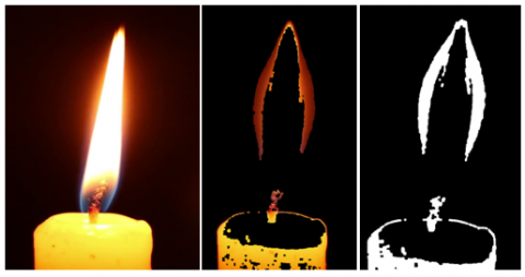
To improve the recognition accuracy, this paper further tests on whether the proposed dynamic features can reduce false positive under the interference of flame photometry and smoke. As shown in Figure 7, our dynamic feature method can provide more physical features for fire recognition. The reason is that the RGB color space is transformed into multiple single spectral spaces. With different features, the detected temperature distribution blocks can be quickly estimated by the two-color high temperature method. In Figure 7, the left subgraph is the recognized area; the center subgraph is the temperature distribution estimated by dynamic features, such that the model can learn deep information of forest fire images; the right subgraph is the RGB black-and-white mode. Obviously, our method mapped very realistic temperature distribution. Of course, there is a certain limitation of our method: the difficulty in handling the scenario of smoldering, which does not emit bright lights but faces smoke interference.
Figure 7. Temperature distribution in the detection area
6.4 Graph visualization
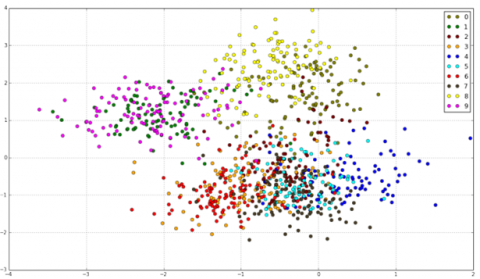
The GNN nodes were classified and visualized on the collected dataset. As shown in Figure 8, each node corresponds to a node in the graph, and its color corresponds to the node class. It can be observed that the nodes of some classes were clustered, while those of other classes were dispersed. For example, Class-1 (magenta) and Class-9 (green) belong to the same cluster. Therefore, they approach each other, but stay away from other classes. This is the result of the similarity guidance by the dynamic features of multi-view images.
Each image could be approximately classified according to the node relationship features between multi-view images and library images. Some points of different colors overlapped each other, suggesting that these relationship features can well update the information of other nodes. The similarity between images from different sources was also considered, and used to update the dynamic features of the library, creating graph nodes of different classes. However, the points of different colors were classified excellently. This means our framework does well in learning the correlations and differences of images from different sources and views.
Figure 8. Visualization of GNN nodes
This paper firstly proposes a GNN based on the similarity of multi-view forest fire images, which successfully estimates the similarity between images. Then, a dynamic feature method was proposed to segment the fire areas from images. This method simplifies the complex preprocessing of images, and effectively extracts the key features of images, enhancing the robustness of forest fire recognition. In addition, a self-made forest fire image dataset was contributed. The experiments on the dataset show that our method applies to various fire scenes, and achieves good generalization and anti-interference abilities, compared to several DL methods. The future research will design a fire recognition and monitoring system with dynamic views, e.g., regularly patrol and flame monitoring by unmanned aerial vehicles (UAVs) in forests.
This work was supported by The Science and Technology Research Program of Chongqing Municipal Education Commission under Grant No.: KJQN202003501.
Di Wu and Chunjiong Zhang have equal contribution to this work.
[1] Xian, J.H., Xu, W., Long, C., Song, Q., Yang, S. (2020). Early forest-fire detection using scanning polarization lidar. Applied Optics, 59(28): 8638-8644. https://doi.org/10.1364/AO.399766
[2] Heyns, A., Plessis, W., Kosch, M., Hough, G. (2019). Optimisation of tower site locations for camera-based wildfire detection systems. International Journal of Wildland Fire, 28(9): 651-665. https://doi.org/10.1071/WF18196
[3] Aslan, Y.E., Korpeoglu, I., Ulusoy, Ö. (2012). A framework for use of wireless sensor networks in forest fire detection and monitoring. Computers, Environment and Urban Systems, 36(6), 614-625. https://doi.org/10.1016/j.compenvurbsys.2012.03.002
[4] Barmpoutis, P., Papaioannou, P., Dimitropoulos, K., Grammalidis, N. (2020). A review on early forest fire detection systems using optical remote sensing. Sensors, 20(22): 6442. https://doi.org/10.3390/s20226442
[5] Saulskii, V.K. (2020). Choosing the structure of satellite systems for meteorology and forest fire detection on the basis of a vector model of surveying the earth. Cosmic Research, 58(4): 295-306. https://doi.org/10.1134/S0010952520040085
[6] Noureddine, H., Bouabdellah, K. (2020). Field experiment testbed for forest fire detection using wireless multimedia sensor network. International Journal of Sensors Wireless Communications and Control, 10(1): 3-14. https://doi.org/10.2174/2210327909666190219120432
[7] Zhang, Z., Zhang, C., Li, M., Xie, T. (2020). Target positioning based on particle centroid drift in large-scale WSNs. IEEE Access, 8: 127709-127719. https://doi.org/10.1109/ACCESS.2020.3008373
[8] Tan, Y.K., Panda, S.K. (2011). Self-autonomous wireless sensor nodes with wind energy harvesting for remote sensing of wind-driven wildfire spread. IEEE Transactions on Instrumentation and Measurement, 60(4): 1367-1377. https://doi.org/10.1109/TIM.2010.2101311
[9] Cao, Y., Yang, F., Tang, Q., Lu, X. (2019). An attention enhanced bidirectional LSTM for early forest fire smoke recognition. IEEE Access, 7: 154732-154742. https://doi.org/10.1109/ACCESS.2019.2946712
[10] Kaliyamurthi, B., Palanisamy, A. (2021). Geographic routing with hybrid firefly algorithm and galactic swarm optimization for efficient ‘void’ handling in mobile ad hoc networks. International Journal of Communication Systems, 34(3): e4690. https://doi.org/10.1002/dac.4690
[11] Wang, Z., Erb, A.M., Schaaf, C.B., Sun, Q., Liu, Y., Yang, Y., Shuai, Y.M., Casey, K.A., Román, M.O. (2016). Early spring post-fire snow albedo dynamics in high latitude boreal forests using Landsat-8 oli data. Remote Sensing of Environment, 185: 71-83. https://doi.org/10.1016/j.rse.2016.02.059
[12] Barmpoutis, P., Stathaki, T., Dimitropoulos, K., Grammalidis, N. (2020). Early fire detection based on aerial 360-degree sensors, deep convolution neural networks and exploitation of fire dynamic textures. Remote Sensing, 12(19): 3177. https://doi.org/10.3390/rs12193177
[13] Arrue, B.C., Ollero, A., De Dios, J.M. (2000). An intelligent system for false alarm reduction in infrared forest-fire detection. IEEE Intelligent Systems and Their Applications, 15(3): 64-73. https://doi.org/10.1109/5254.846287
[14] Sudhakar, S., Vijayakumar, V., Kumar, C.S., Priya, V., Ravi, L., Subramaniyaswamy, V. (2020). Unmanned Aerial Vehicle (UAV) based Forest Fire Detection and monitoring for reducing false alarms in forest-fires. Computer Communications, 149: 1-16. https://doi.org/10.1016/j.comcom.2019.10.007
[15] Jilbab, A., Bourouhou, A. (2020). Efficient forest fire detection system based on data fusion applied in wireless sensor networks. International Journal on Electrical Engineering and Informatics, 12(1): 1-18. http://dx.doi.org/10.15676/ijeei.2020.12.1.1
[16] Qin, L., Wu, X., Cao, Y., Lu, X. (2019). An effective method for forest fire smoke detection. Journal of Physics: Conference Series, 1187: 052045. http://dx.doi.org/10.1088/1742-6596/1187/5/052045
[17] Kingma, D., Ba, J. (2014). Adam: A method for stochastic optimization. Computer Science. http://arxiv.org/abs/1412.6980v8
[18] Jeong, S.W., Yoo, J. (2020). I-firenet: A lightweight CNN to increase generalization performance for real-time detection of forest fire in edge AI environments. Journal of Institute of Control, 26(9): 802-810. http://dx.doi.org/10.5302/J.ICROS.2020.20.0033
[19] Sun, X., Sun, L., Huang, Y. (2020). Forest fire smoke recognition based on convolutional neural network. Journal of Forestry Research, pp. 1-7. https://doi.org/10.1007/s11676-020-01230-7
[20] Dubey, V., Kumar, P., Chauhan, N. (2019). Forest fire detection system using IoT and artificial neural network. In International Conference on Innovative Computing and Communications (pp. 323-337). Springer, Singapore. https://doi.org/10.1007/978-981-13-2324-9_33
[21] Attri, V., Dhiman, R., Sarvade, S. (2020). A review on status, implications and recent trends of forest fire management. Archives of Agriculture and Environmental Science, 5(4): 592-602. https://doi.org/10.26832/24566632.2020.0504024
[22] Cuomo, V., Lasaponara, R., Tramutoli, V. (2001). Evaluation of a new satellite-based method for forest fire detection. International Journal of Remote Sensing, 22(9): 1799-1826. https://doi.org/10.1080/01431160120827
[23] Hammad, M., Pławiak, P., Wang, K., Acharya, U.R. (2020). ResNet-Attention model for human authentication using ECG signals. Expert Systems, e12547. https://doi.org/10.1111/exsy.12547
[24] Alkhatib, A.A. (2014). A review on forest fire detection techniques. International Journal of Distributed Sensor Networks, 10(3): 597368. https://doi.org/10.1155/2014/597368
[25] Wang, L., Qu, J.J., Hao, X. (2008). Forest fire detection using the normalized multi-band drought index (NMDI) with satellite measurements. Agricultural and Forest Meteorology, 148(11): 1767-1776. https://doi.org/10.1016/j.agrformet.2008.06.005
[26] Zhang, C., Xie, T., Yang, K., Ma, H., Xie, Y., Xu, Y., Luo, P. (2019). Positioning optimisation based on particle quality prediction in wireless sensor networks. IET Networks, 8(2): 107-113. https://doi.org/10.1049/iet-net.2018.5072
[27] Rahim, T., Khan, S., Arslan, M., Shin, S.Y. (2020). Exploiting de-noising convolutional neural networks DnCNNs for an efficient watermarking scheme: A case for information retrieval. IETE Technical Review, 38(2): 245-255. https://doi.org/10.1080/02564602.2020.1721342
[28] Fu, S., Yang, X., Liu, W. (2018). The comparison of different graph convolutional neural networks for image recognition. In Proceedings of the 10th International Conference on Internet Multimedia Computing and Service, pp. 1-6. https://doi.org/10.1145/3240876.3240915
[29] Mukherjee, A., Rai, R., Singla, P., Singh, T., Patra, A. (2015). Laplacian graph based approach for uncertainty quantification of large scale dynamical systems. In 2015 American Control Conference (ACC), pp. 3998-4003. https://doi.org/10.1109/ACC.2015.7171954
[30] Yuan, C., Liu, Z., Zhang, Y. (2016). Vision-based forest fire detection in aerial images for firefighting using UAVs. In 2016 International Conference on Unmanned Aircraft Systems (ICUAS), pp. 1200-1205. https://doi.org/10.1109/ICUAS.2016.7502546
[31] Culjak, I., Abram, D., Pribanic, T., Dzapo, H., Cifrek, M. (2012). A brief introduction to OpenCV. In 2012 Proceedings of the 35th International Convention MIPRO, IEEE, pp. 1725-1730.
[32] Bai, Y., Hu, J., Su, J., Liu, X., Liu, H., He, X., Meng, S.W., Mas, E., Koshimura, S. (2020). Pyramid pooling module-based semi-Siamese network: A benchmark model for assessing building damage from xBD satellite imagery datasets. Remote Sensing, 12(24): 4055. https://doi.org/10.3390/rs12244055