Yong Chen* | Yanyan Wang | Zihong Cai | Mian Jiang
© 2021 IIETA. This article is published by IIETA and is licensed under the CC BY 4.0 license (http://creativecommons.org/licenses/by/4.0/).
OPEN ACCESS
The diagnosis of central lymph node metastasis (CLNM) is very important for the treatment of papillary thyroid carcinoma (PTC), which remains highly subjective and depends on clinical experience. Traditional method based on radiomics tumor feature (RTF) extraction and classifications has its shortages to predict the CLNM and increase the possibility of over-diagnosis and over-treatment leading for PTC. In this paper, a convolutional neural network (CNN) based fusion modeling method is proposed for predictions of CLNM in ultrasound-negative patients with PTC. A CNN and a RTF extraction based random forest (RF) classifier are trained on the context image patches and tumor image patches, and the probability outputs from these two models are combined for predicting the CLNM. It is validated that the proposed method has better diagnostic performance than the conventional method on the test set. The area under the curve (AUC), accuracy, sensitivity, and specificity of the method in predicting CLNM are 0.9228, 83.09%, 86.17%, and 81.46%, respectively. It has the prospect to apply to diagnose ultrasound (US) images with the machine-learning diagnostic system.
papillary thyroid carcinoma, central lymph node metastasis, ultrasound images, radiomic feature, deep learning, convolutional neural network
Thyroid cancer has 58,600 cases worldwide, ranking ninth in the incidence of cancer in 2018.PTC accounts for the vast majority of all thyroid cancers (>90%) [1]. Although the malignant degree of thyroid carcinoma is relatively low, local invasion and distant metastasis can also occur [2, 3]. The guidelines published by American Thyroid Association (ATA) indicate that selective central lymph node dissection (CLND) can be performed [4]. However, studies have shown no long-term additional benefit from prophylaxis of central lymph node dissection (pCND), with temporary and permanent hypoparathyroidis-related complications of 30% and 5%-10% respectively, and a higher rate of nerve damage associated with pCND [5].
Medical image processing algorithm is an interdisciplinary application of medical field and computer vision field which is widely used in recent years. Using the ability of computer image processing can help clinicians judge whether patients are sick or not, so as to improve the accuracy of diagnosis and prediction results. In recent years, the cross fusion of computer technology and medical image-assisted diagnosis has produced a new radiomics, which can effectively solve the problem of tumor evaluation by extracting a large number of features from the image to quantify the tumor [6]. Some researchs have attempted to use radiomics to predict PTC central lymph node metastasis, but the accuracy is only 4% higher than random probability [7].
In addition, with the development of deep learning (DL), some researchers try to apply DL to medical images in the prediction of lymph node metastasis (LNM). In this paper, DL is applied in the prediction of LNM of primary breast cancer and the final AUC is 0.89, which proves that the DL model can effectively predict negative LNM [8]. However, DL needs a large amount of data as a support, and it is difficult to obtain enough high-quality data sets in the field of PTC of CLNM. Failure to obtain enough data sets greatly limits the exploration and application of DL in the field of thyroid nodule images. Most importantly, PTC ultrasound images have very small differences, and it is difficult to detect the features of CLNM, which is very unfriendly to DL methods. Radiomics can solve this problem, because DL pays attention to the information of thyroid tissues, and radiomics is more sensitive to the features of focal regions. Although many studies have focused on the prediction of LNM by radiomics, its accuracy is not high and the effect is not good.
In view of the above difficulties, in order to solve the shortcomings of insufficient PTC of US image data, data enhancement and transfer learning methods are proposed. The model based on the combination of radiomics and DL is proposed to extract the information of PTC lesion and the tissue information around thyroid nodule at the same time.
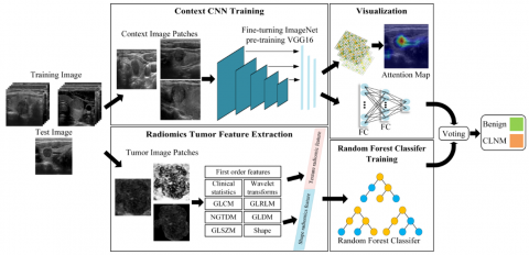
As shown in Figure 1, the proposed method is a combination of a context CNN model (VGG16) and a RTF model to predict CLNM in US-negative PTC. In RF-based RTFmethods [9], a patch image which cropped around the tumor is used for the radiomics feature extraction, instead of the entire image, as a the primary means of reflecting the tumor information. In patch generation, information trade-off occurs depending on the ratio of the tumor size to the patch size. If most of the patch region is occupied by the tumor, the intra tumoral texture information can be reflected well, but the context information between the tumor and the organ is largely ignored. In contrast, if the patch includes not only the tumor but also some parts of the organs, the context information for VGG16 would be strengthened, but the reflection of the intra tumoral information would be weakened. A framework is proposed to utilize both types of information by training both types of patches and combine them.
The method proposed in this paper includes three main steps: (1) radiomics feature extraction and RF classification on tumor image patches, (2) CNN model training and classification on context image patches, and (3) two types of classification probability weighted fusion to get the final result. The validity of the predictions provided by this model are verified by comparison with biopsy results. The data of 906 ultrasound-negative patients with PTC have been collected from January 2016 to May 2019. It is verified that the model can assist doctors in accurately predicting CLNM with US-negative PTC. This will aid in the design of treatment regimens and reduce the occurrence of unnecessary diagnostic dissection for patients without metastasis, thereby reducing the associated risk of complications.
The remainder of this paper is organized as follows: Section 2 describes the characteristics and classification of radiomics, Section 3 describes the CNN-based fusion model, Section 4 introduces the verification and discussion of the model and Section 5 is the conclusion.
Figure 1. Flow diagram of the method
2.1 Data pre-processing
First, the PTC in the US image is manually segmented by a clinician with 10 years of experience using ITK-SNAP software, and the region of interest (ROI) of the PTC lesion is obtained automatically by programming. Then, the ROI is transformed into the Fourier frequency domain to obtain the low-frequency and high-frequency components [10]. After transformation, most of the energy is concentrated in the low-frequency component, while the detail is in the high-frequency component. The image is sharpened using a Gaussian high-pass filter [11], the transfer is used as shown in formula (1).
$H(u, v)=1-e^{-D^{2}(u, v) / 2 D_{0}^{2}}$ (1)
where, D0 is the specified non-negative number, D(u, v) is the center distance from the point (u, v) to the filter.
To enhance the contrast and highlight the detailed information, the low-frequency and high-frequency components are weighted at the same time. However, the weighting coefficient of the low-frequency component must be less than that of the high-frequency one to ensure that the low-frequency component will not be lost, and the edge details of the high-frequency component are significantly enhanced. The transfer function of the high-frequency emphasis filter is shown as formula (2).
$H_{h f e}(u, v)=a+b H_{h p}(u, v)$ (2)
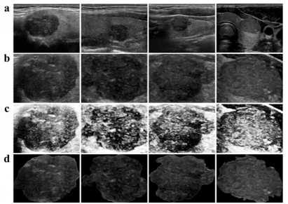
Finally, the inverse Fourier transformation is carried out in the spatial domain, and then histogram equalization is used to improve the brightness and contrast and highlight the features of the thyroid ROI. The tumor image patch is generated as a squared patch circumscribing the tumor as the conventional image patch for the tumor classifying RTF inputs. The generated tumor image patch can reflect the intra tumoral texture and tumor shape information to the RTF training.where, a is the offset, b is the multiplier, and Hhp(u, v) is the Gaussian high-pass filter transfer function.
The procedure of the pre-processing is shown in Figure 2. (a) is the original figure of PTC, and (b) is a map of the focus manually segmented by the clinician, (c) is the focus map after high frequency emphasis filtering and histogram equalization, and (d) shows the internal outline of the focus.
Figure 2. Data pre-processing
2.2 Feature extraction
For the image segmentation, this paper uses the gold standard of manual segmentation for the input of this method. The descriptions are summarized as 577 features. The features of this method are divided into nine categories: clinical statistical information, first-order features, gray level co-occurrence matrix features, gray level size zone matrix features, gray level run length matrix features, gray level dependence matrix features, neighboring gray-tone difference matrix features, shape features, and wavelet transforms. All imaging features can be divided into three categories [6, 12, 13].
2.2.1 First-order statistical characteristics
The first-order statistical feature is mainly the basic statistics describing the numerical distribution of pixels. As shown in formula (3) and (4) , X is used to represent the image, N is the number of pixels, Xi is the discrete gray intensity of i position, and $\bar{X}$ is the mean value of X, the gray histogram is the description of the surface layer of the image, and the features extracted from the histogram are invariant, such as scale and displacement and rotation, the histogram of each PTC is calculated from the ultrasound image, and the first-order statistical feature (mean, standard deviation (SD), skewness, and kurtosis) are calculated easily.
Moreover, the percentile-mean and percentile standard deviation (percentile-SD) are also derived from the first 50%, 25%, and 10% of the histogram curve.
Where, α represents the percentile (50%, 25% and 10%) and M is the number of pixels in the unselected (1-α) part.
$\operatorname{mean}_{\alpha}=\frac{1}{N-M} \sum_{i=M}^{N}\left(X_{i}-\bar{X}\right)^{2}$ (3)
$S D_{\alpha}=\sqrt{\frac{1}{N-M} \sum_{i=1}^{N}\left(X_{i}-\bar{X}\right)^{2}}$ (4)
2.2.2 Texture feature
Table 1 mainly defines the following general expressions, and then calculates the statistics.
The texture feature is mainly for extracting the texture feature of the gray level cooccurrence matrix (GLCM), defining the GLCM as a matrix with Ng×Ng and recorded as P(i, j, δ, θ). This matrix represents the second-order joint probability function of the image. Here, (i, j) is the number of times that a combination of i and j appear. These pixels are all with a distance of $\delta \text { in the } \theta$ direction.
Table 1. Expressions and their meanings
|
Expression |
Meanings |
|
P(i,j) |
Gray level co-occurrence matrix of arbitrary θ and δ |
|
μ |
The mean value of P(i,j) |
|
μx(i) |
The mean value of Px(i) |
|
μy(j) |
The mean value of Py(j) |
|
σx(i) |
The standard deviation of Px(i) |
|
σy(j) |
The standard deviation of Py(j) |
(1) Energy is the square sum of the elements in the gray co-occurrence matrix, which can reflect the uniformity of texture grayscale, reflect the texture thickness of the image distribution, and quantify the uniformity of the grayscale. It is shown in formula (5) .
$\text { energy }=\sum_{i=1}^{N_{g}} \sum_{j=1}^{N_{g}} P(i, j)^{2}$ (5)
(2) Contrast is a statistic of texture thickness which reflects the uniform gray distribution of the image. It can describe the numerical distribution and local variation of the matrix. It can also reflect the clarity and groove depth, and count the change of local strength. It is shown in formula (6).
$\text { contrast }=\sum_{i=1}^{N_{B}} \sum_{j=1}^{N_{g}}|i-j|^{2} P(i, j)$ (6)
(3) Correlation is used to calculate the gray correlation of a specified location, and the correlation is mainly to calculate the degree of similarity between elements in rows or columns. It is shown in formula (7).
$\text { correlation }=\frac{\sum_{i=1}^{N_{g}} \sum_{j=1}^{N_{g}} i j P(i, j)-\mu_{x}(i) \mu_{y}(j)}{\sigma_{x}(i) \sigma_{y}(j)}$ (7)
(4) Entropy describes the uniformity of the image and quantifies the randomness of the texture. The more uniform the image, the greater the entropy. It is shown in formula (8).
$\text { entropy }=\sum_{i=1}^{N_{g}} \sum_{j=1}^{N_{g}} P(i, j) \log _{2} P(i, j)$ (8)
(5) Homegeneity is a statistic that describes local changes and reflects the homogeneity of texture. It is inversely proportional to the contrast weight, and the larger the value is, the smaller the local change is, that is, the more uniform the local is. It is shown in formula (9).
$\text { homegenity }=\sum_{i=1}^{N_{g}} \sum_{j=1}^{N_{g}} \frac{P(i, j)}{1+|i-j|^{2}}$ (9)
2.2.3 Shape features
Shape features are expected to describe the shape-related features of the lesions, including the area, perimeter, and maximum diameter of the lesions. These features can get the objective description of the focus, which is the feature extraction of the surface information of the image.
Npixels is the number of 1 in the ROI, and LPS denotes the number of pixels of the focus. The calculating area is $A=N_{\text {pixels }} L_{P S}^{2}$, the circumference is $C=N_{\text {pixels }} L_{P S}$. Max diameter refers to the maximum Euclidean distance in pairs of pixels in the ROI region. The circumference to area ratio is the ratio of the perimeter to the area, $R_{C / A}=\frac{C}{A}$, the circular disproportion is $C D=\frac{C}{2 \pi R}$, and the roundness is $\text { roundness }=\frac{4 \pi A}{C^{2}}$.
All features are extracted from the original US-negative PTC images [14]. The relationship between lymph node status and imaging features is explored by machine learning.
Table 2 shows a part of the radiomics features extracted by machine learning.
Table 2. Radiomics features extracted by machine learning
|
Label |
Age |
Size (mm) |
Piexl (mm) |
Area (10mm2) |
MaxFeretDiameter (mm) |
MinFeretDiameter (mm) |
|
1 |
18 |
16.4 |
0.07066455 |
1770.288317 |
16.79052767 |
10.09166174 |
|
0 |
77 |
19.2 |
0.079379845 |
2260.499845 |
18.08693762 |
13.9567339 |
|
1 |
56 |
25 |
0.059210526 |
1964.960526 |
20.80607681 |
13.08438549 |
|
0 |
36 |
12.1 |
0.061813187 |
1693.372253 |
14.78899064 |
10.22310505 |
|
0 |
27 |
19 |
0.070532915 |
4787.210031 |
28.49328999 |
15.48598436 |
|
0 |
43 |
3 |
0.079470199 |
260.6622517 |
9.142182022 |
4.137641687 |
|
1 |
33 |
12.4 |
0.070874862 |
1862.024363 |
15.86235772 |
12.15117709 |
|
0 |
30 |
3 |
0.070532915 |
410.9952978 |
10.04691802 |
5.285984116 |
|
0 |
35 |
4 |
0.085714286 |
132.5142857 |
5.990809287 |
3.106278051 |
|
0 |
38 |
4 |
0.069767442 |
445.8837209 |
11.71179046 |
5.454636659 |
|
0 |
44 |
10.4 |
0.09375 |
458.34375 |
9.685786139 |
6.653979771 |
|
1 |
46 |
12.1 |
0.079817362 |
478.9041741 |
10.51076778 |
5.989515158 |
|
1 |
43 |
17 |
0.085551331 |
2239.990494 |
18.67391748 |
14.54372624 |
|
0 |
49 |
14 |
0.088235294 |
1715.735294 |
18.79970919 |
14.0073867 |
|
0 |
29 |
10.9 |
0.0593 |
1215.7686 |
12.65857086 |
8.99072946 |
|
1 |
26 |
4 |
0.079817362 |
196.0314419 |
5.827214121 |
4.220164743 |
|
1 |
41 |
15.3 |
0.058823529 |
3423.176471 |
20.66121519 |
13.05120308 |
|
1 |
35 |
17.4 |
0.070754717 |
3198.466981 |
23.96256592 |
14.46655605 |
2.3 Model reduction and the RF-based classifier
There are 577 groups of clinical features and image features. Because of the repeatability and redundancy of image group features, dealing with high-dimensional features requires more memory and processing power. Principal component analysis (PCA) can synthesize high-dimensional variables that may have correlation to linearly independent low-dimensional variables to alleviate dimensional disaster problems. At the same time, dimensionality reduction can minimize information loss while compressing data.
The PCA is employed to reduce the dimensions of the data, and can keep only the terms corresponding to the K largest eigenvalues. Hence, this obtains a new feature vector consisting of eigenvectors of principal components. The final data computed using this feature vector and the mean adjusted original input data is obtained as shown in formula (10).
$F_{\text {data }}=R F_{\text {vector }} \times R D_{\text {adjust }}$ (10)
where, RFvector is the matrix in which eigenvectors in the columns are transposed and RDadjust is the mean adjusted input data. Fdata is the characteristic matrix after PCA dimension reduction. The obtained subspace is spanned by the orthogonal set of eigenvectors which reveal the maximum variance in the data space.
Using PCA mapping high-dimensional data into low dimensional data reduces the calculation cost of NIDS and improves the efficiency of the analysis. Here, PCA has been used for dimensionality reduction of the forty-two dimensions and the output of the PCA method provides a set of features that are the linear combination of the original set of features. PCA provides RF with the features that allow for efficient classification from an informative view point. Then, the RFclassifier [15, 16] is used in this method and 100 trees are employed in each RF. Data enhancement is performed on the training set to reduce deviation and overfitting.
Different features according to the type of input image can be obtained because of the different training methods described above. The model trained with tumor image patches mainly learns the correlation between texture information and clinical information, while the VGG16 model trained with context image patches mainly learns the relationship of context information.
Based on the learning properties of different models, in addition to evaluating the performance of the CNN and RTF model, the performance of a combination of these two models (combined model) is evaluated. The prediction of the fusion model is the combination of the outputs of VGG16 and RTF models. The combination coefficient of the two models is set to be 0.5, which can be modified according to different situations. The above methods are used to evaluate the performance by evaluating the AUC, accuracy, sensitivity, and specificity.
3.1 Typical CNN model: VGG16
The most representative of the deep learning models is deep CNN, which usually consists of one or more layers including the convolution layer, activation layer (Relu), pooling layer, and full connection layer. VGG16 is a typical deep CNN model. Because the amount of data is relatively small, VGG16 has better migration performance, so it is suitable to be used.
Table 3 shows the detailed parameters of the VGG16 network. VGG16 has 16 hidden layers. The input size of the network is 224×224 RGB images, and the convolution core of each convolution layer in the network is 3×3. After the image data is processed by the convolution layer and pooling layer, the size of the feature image decreases gradually, while the depth increases continuously. The final feature image size is 7×7, and the number of channels is 512.
The VGG network uses a smaller 3×3 convolution kernel, while two consecutive 3×3 convolution kernels are equivalent to 5×5 receptive fields. This change results in a smaller number of parameters, saving computing resources and leaving resources to a deeper network.
The calculation process of the VGG16 model can be expressed by formula (11).
$y(n+1)=\operatorname{vgg}(y(n) \cdot x(n))$ (11)
where, n represents the number of layers of the network, y(n) represents the output of the nth layer, y(0) is the input, x(n) represents the convolution kernel matrix at layer n, and vgg(.) is the function of the VGG network.
Table 3. Detailed parameters of VGG16
|
Model: "vgg16" |
||
|
Layer (type) |
Output Shape |
Param # |
|
input_1 (InputLayer) |
[(None, 224, 224, 3)] |
0 |
|
block1_conv1 (Conv2D) |
(None, 224, 224, 64) |
1792 |
|
block1_conv2 (Conv2D) |
(None, 224, 224, 64) |
36928 |
|
block1_pool (MaxPooling2D) |
(None, 112, 112, 64) |
0 |
|
block2_conv1 (Conv2D) |
(None, 112, 112, 128) |
73856 |
|
block2_conv2 (Conv2D) |
(None, 112, 112, 128) |
147584 |
|
block2_pool (MaxPooling2D) |
(None, 56, 56, 128) |
0 |
|
block3_conv1 (Conv2D) |
(None, 56, 56, 256) |
295168 |
|
block3_conv2 (Conv2D) |
(None, 56, 56, 256) |
590080 |
|
block3_conv3 (Conv2D) |
(None, 56, 56, 256) |
590080 |
|
block3_pool (MaxPooling2D) |
(None, 28, 28, 256) |
0 |
|
block4_conv1 (Conv2D) |
(None, 28, 28, 512) |
1180160 |
|
block4_conv2 (Conv2D) |
(None, 28, 28, 512) |
2359808 |
|
block4_conv3 (Conv2D) |
(None, 28, 28, 512) |
2359808 |
|
block4_pool (MaxPooling2D) |
(None, 14, 14, 512) |
0 |
|
block5_conv1 (Conv2D) |
(None, 14, 14, 512) |
2359808 |
|
block5_conv2 (Conv2D) |
(None, 14, 14, 512) |
2359808 |
|
block5_conv3 (Conv2D) |
(None, 14, 14, 512) |
2359808 |
|
block5_pool (MaxPooling2D) |
(None, 7, 7, 512) |
0 |
|
Total params: 14,715,714 Trainable params: 7,080,450 Non-trainable params: 7,635,264 |
||
The VGG network has outstanding expansion performance and simple structure, so it has good migration performance and good generalization performance when migrating to other data sets. The VGG16 network structure diagram is shown in Figure 3. The structure of the VGG16 network is very simple, while at the same time delivers a good effect. Its appearance verifies that the performance can be improved by deepening the number of layers of the network.
Figure 3. Network structure of VGG16
3.2 Data augmentation and transfer learning
The context image patch is generated as a square patch containing the tumor and the information of the nearby tissues. The generated context image patch can reflect the context information between the tumor and the neck tissue status, such as the relative location of the tumor in the neck and the PTC information itself, in order to solve the data imbalance [8]. Hence, data augmentation is also performed on the training set to generate 2,000 images for each class by rotation, scaling, and filtering, and then focusing on context information to prevent overfitting. Then, the size of images (224 × 224 pixels) is adjusted to normalize the distance scale. These images are used as input for the training of the VGG16 model [17].
DL has the ability to represent learning, which automatically identifies features that are relevant for a particular task from the original data. Deep learning is a new research direction in the field of machine learning, which can obtain enough data in various fields. With the support of sufficient data, deep learning can bolster traditional machine learning. However, it is difficult to obtain enough medical imaging data due to various restrictions. In this case, transfer learning can allow deep learning to still obtain sufficient performance on insufficient data sets. Transfer learning is a more efficient and reliable method for small data classification applications of DL [18, 19]. The transfer learning method proposed is based on VGG16.
The architecture of the VGG16 model consists of five stacks, each of the stacks contains two convolution layers, which consists of a maximum pool layer and three fully connected layers. The model is pre-trained using the ImageNet database and fine-tuned using a given data set [7]. Transfer learning is performed at learning rate of 1e-4, batch size of 4, and maximum epochs is 120. CNN features are extracted from the first, third, and fifth max-pool layers, which are then average-pooled along spatial dimensions, resulting in three feature vectors. Each of the three vectors are individually normalized and concatenated with a fully connected layer to form a final CNN feature vector, which is then normalized again.
3.3 Visualization
Because the model is created to predict whether or not CLNM occurs, the model is designed to learn the context image and predict CLNM. It is known that the peripheral shape and depth texture signals of PTC are related to CLNM. Therefore, feature visualization is used to determine if attention is allocated in and around PTC [20].
Class activation mapping uses a two-dimensional fractional network associated with a specific output category, which calculates each location of the input image and indicates how important each location is to that category. Class activation map visualization can help in understanding of which part of an image makes the convolution neural network make the final classification decision. This is helpful to debug the decision-making process of the convolution neural network, especially in the case of misclassification. The procedure of visualization is given as follows [21, 22].
(1) Specify a picture to be classified and input it to the model and preprocess it. Load the VGG19 network that has been set up and load the specified picture to be classified.
(2) Obtain the gradient of the model output relative to the active output of the last convolution layer. The activation output of the last convolution layer is obtained by using the model.get_layer function, and the gradient of the model output for the last convolution layer activation output is calculated by using the K.gradients function.
(3) Characterize the importance of each point of the final convolution layer activation output to the model decision classification and use pre-processing to obtain the class activation graph. The K.mean function is used to homogenize the gradients, and the K.function function is used to establish the functional relationship among the model output, the last convolution layer activation output, and the gradient mean. The gradient value is multiplied by the eigenvalues of each channel in the last convolution layer, and the product is used to express the importance of each point to the final classification decision of the model, that is, the class activation map.
(4) Render the adjusted convolution activated output as a thermal effect.
(5) The original image is superimposed with the rendered thermal map prior to visualization.
Python scripting language is used and python libraries such as numpy and openCV2 are required in the experiments. The experiments are designed and implemented by tensor flow deep learning framework and compiled by pycharm compiler. The computer hardware configuration is as follows: the GPU is GeForce GTX 1080Ti with 12G video memory, the CPU is Intel (R) Core (TM) i7-6850K, the main frequency is 3.60GHz, the memory size is 64G. The manual marking ultrasound image software used is ITK-SNAP3.8.0 and the statistical software is SPSS26.0.
4.1 Data selection
This retrospective research protocol has been approved by the Ethics Review Board of the Department of Ultrasound at Sun Yat-sen University Cancer Center. Written informed consent from all participants has been obtained. All of the procedures are performed in accordance with the Declaration of Helsinki and relevant policies in China.
The participants include 906 consecutive patients who underwent near, sub-, or total thyroidectomy, and have been pathologically confirmed with PTC by the Department of Head and Neck in the hospital between January 2016 and May 2019.The inclusion criteria for the thyroidectomy are: (a) patients ≥18 years old, and (b) no clear CLN identified from US images. The exclusion criteria are: (a) patients who previously underwent a neck operation, (b) patients diagnosed with other types of thyroid tumor at the same time, (c) patients with a previous history of radiation therapy, and (d) patients who are unavailable to be completely evaluated by US. Patient enrolment details are shown in Figure 4. In the center, surgical procedures are performed on patients based on the recommendation of the National Comprehensive Cancer Network and the American Thyroid Association. Prophylactic CLND is commonly performed in the VI compartment (neck level VI) according to the institutional protocol, regardless of the clinical evidence of CLNM. Prophylactic CLND is typically perforated.
Clinical data, such as age, gender, and other basic patient information, are collected from the electronic medical records in the registry. Pathologic information is gathered from postoperative pathology reports in the electronic medical record. All diagnoses are rendered and reported by pathologists with 7–20 years of experience.
A comprehensive neck US examination is preoperatively performed on all the patients in the supine position, with their neck extended, using a 5–18 MHz linear array transducer machine (iU22, Philips Medical Systems; Acuson Sequoia 512, Siemens Medical Solutions; LOGIQ S8 and E9, GE Medical Systems). These tests are performed by board-certified doctors with 7–20 years of experience, specializing in head and neck imaging. The doctor who performed the US examination prospectively records the US features of the thyroid nodule and CLN status. If more than one nodule under suspicion of malignancy has been found in the thyroid gland, the maximum diameter of the most suspicious lesion is recorded and included in the data analysis.
Figure 4. Patient enrolment details
4.2 Results analysis
4.2.1 Nodule characteristics
All 906 patients are confirmed to have PTC by surgical pathology in the Sun Yat-sen University Cancer Center from January 2016 to May 2019, among which 322 cases are CLNM positive and 584 cases involved metastasis. The PTC diagnosis is based on the final pathology results. The 634 cases (about 70%) in the training set have a median age of 42.76 years (in the range of 18-74), and include 191 males (30.13%) and 443 females (69.87%), where 228 cases (35.96%) are CLNM positive. Further, 196 cases in the validation set (about 30%) have a median age of 44.30 years (in the range of 18–79), and include 93 males (34.19%) and 179 females (65.81%), where 94 cases (34.56%) are CLNM positive. No significant difference is found in demographic profiles between the two groups.
Eight features are listed based on clinical and US features. Univariate analysis shows that CLNM is related to sex, age, tumor size, microcalcification, extra-thyroid invasion, shape, vascular invasion, and aspect ratio. These eight features are identified as the key factors and are discussed considering the manual extraction of features (Table 4; P<0.001).
Table 4. Relationship between clinical and US characteristics
|
Modeling |
Training Total |
CNM(−) |
CNM(+) |
P value |
Validation Total |
CNM(−) |
CNM(+) |
P value |
|
N=634 |
N=406 |
N=228 |
N=272 |
N=178 |
N=94 |
|||
|
Gender |
|
|
|
<0.001 |
|
|
|
<0.001 |
|
Male |
191(30.13%) |
104(25.62%) |
87(38.16%) |
|
93(34.19%) |
41(23.03%) |
51(54.26%) |
|
|
Female |
443(69.87%) |
302(74.38%) |
141(61.84%) |
|
179(65.81%) |
137(76.97%) |
43(45.74%) |
|
|
Age |
|
|
|
<0.001 |
|
|
|
<0.001 |
|
≤45 years |
373(58.83%) |
227(55.91%) |
146(64.04%) |
|
151(55.51%) |
102(57.3%) |
50(53.19%) |
|
|
>45 years |
261(41.17%) |
179(44.09%) |
82(35.96%) |
|
121(44.49%) |
76(42.7%) |
44(46.81%) |
|
|
Tumor size |
|
|
|
<0.001 |
|
|
|
<0.001 |
|
≤1 cm |
307(48.42%) |
222(54.68%) |
84(36.84%) |
|
146(53.68%) |
109(61.24%) |
38(40.42%) |
|
|
1-2 cm |
262(41.32%) |
156(38.42%) |
106(46.49%) |
|
100(36.76%) |
58(32.58%) |
42(44.68%) |
|
|
2-3 cm |
53(8.36%) |
22(5.42%) |
30(13.16%) |
|
20(7.35%)) |
9(5.06%) |
12(12.77%) |
|
|
>3 cm |
12(1.9%) |
6(1.48%) |
8(3.51%) |
|
6(2.21%) |
2(1.12%) |
2(2.13%) |
|
|
Microcalcification |
|
|
|
<0.001 |
|
|
|
<0.001 |
|
No |
242(38.17%) |
179(44.08%) |
62(27.19%) |
|
99(36.4%) |
76(42.7%) |
23(24.47%) |
|
|
Scattered distribution |
319(50.32%) |
188(46.31%) |
131(57.46%) |
|
136(50.0%) |
80(44.94%) |
55(58.51%) |
|
|
Aggregated distribution |
73(11.51%) |
39(9.61%) |
35(15.35%) |
|
37(13.6%) |
22(12.36%) |
16(17.02%) |
|
|
Extra-thyroid invasion |
|
|
|
<0.001 |
|
|
|
<0.001 |
|
No |
145(22.87%) |
110(27.09%) |
35(15.35%) |
|
33(12.13%) |
21(11.8%) |
13(13.83%) |
|
|
Yes |
489(77.13%) |
296(72.91%) |
193(84.65%) |
|
239(87.84%) |
157(88.20%) |
81(86.17%) |
|
|
Shape |
|
|
|
|
|
|
|
|
|
Normal |
337(53.15%) |
209(51.48%) |
129(56.58%) |
|
173(63.6%) |
110(61.80%) |
63(67.02%) |
|
|
Abnormal |
297(46.85%) |
197(48.52%) |
99(43.42%) |
|
99(36.4%) |
68(38.2%) |
31(32.98%) |
|
|
Blurred edge |
|
|
|
<0.001 |
|
|
|
<0.001 |
|
Yes |
311(49.05%) |
191(47.04%) |
120(52.63%) |
|
140(51.47%) |
90(50.56%) |
50(53.19%) |
|
|
No |
323(50.95%) |
215(52.96%) |
108(47.37%) |
|
132(48.53%) |
88(49.44%) |
44(46.81%) |
|
|
Aspect ratio |
|
|
|
|
|
|
|
|
|
≤1 |
120(18.93%) |
93(22.91%) |
28(12.28%) |
|
79(29.04%) |
64(35.96%) |
16(17.02%) |
|
|
>1 |
514(81.07%) |
313(77.09%) |
200(87.72%) |
|
193(70.96%) |
114(64.04%) |
78(82.98%) |
|
4.2.2 Comparison of the predict models
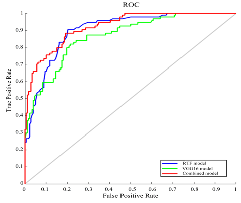
In the validation set, 272 cases are input into the RTF model, the fine-tuned VGG16 model, and the combined model. Table 5 shows the CLN prediction results of the three comparison methods. In the validation set, the VGG16 model shows slightly lower accuracy than the RTF model (78.31% and 81.92%, respectively), although the sensitivity of VGG16 is significantly higher than that of the RTF model. This may be because of the fact that the texture and shape of the tumor are important criteria for predicting CLNM, in addition to the tissue around the tumor. However, compared with the RTF and VGG16 models, the combined model shows an increase sensitivity of13.83% and 3.19%, respectively, and an increase in ACC of 1.17% and 4.78%, respectively.
Table 5. Performance comparison of machine-learning prediction models based on US features
|
Validation data set |
||||
|
Classifier |
Accuracy |
Sensitivity |
Specificity |
AUC |
|
VGG16 model |
78.31% |
82.98% |
75.84% |
0.8668 |
|
RTF model |
81.92% |
72.34% |
87.08% |
0.9052 |
|
Combined model |
83.09% |
86.17% |
81.46% |
0.9228 |
Figure 5 shows the receiver operating characteristic curves(ROC) obtained using the three different models. The AUC of the VGG16 model is slightly lower than that of the RTF model. However, as context and intra-tumor information are complementary for the prediction, the combined model that includes both of these data shows an increase in overall performance, with an AUC value of 0.9228. Hence, the combination of the context VGG16 model and RTF model has a high potential for predicting CLNM in US-negative patients with PTC. The results show that the fusion of the model has the potential to assist CLNM detection.
Figure 5. Receiver operating characteristic curves obtained using the three different models
4.2.3 Visualization effect
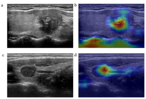
As shown in Figure 6, (b) map is the visualization of (a) map. It can be seen from the figure that the deep convolution network has noticed the focus area and marked it clearly. This shows that the deep convolution network has known the abnormal characteristics of malignant tumors and used them as an important basis for the prediction of central lymph node metastasis. (b) map pays attention not only to the location of the lesion, but also to the edge of the thyroid gland. This shows that the surrounding tissue information is also the basis for the prediction of central lymph node metastasis, and validates that the model studied in this paper not only pays attention to the texture and shape of the focus, but also is sensitive to context information and surrounding tissue information.
Figure 6. Feature visualization
4.3 Discussion
PTC is one of the most common cancers diagnosed in the world, and its main life-threatening manifestations are lymph node metastasis and extra-thyroid spread [4, 23, 24]. The early diagnosis and treatment of CLNM is the most significant means of reducing the mortality and recurrence rate of patients with PTC [25, 26]. US is an effective tool for precise localization of PTC lesions, however, most radiologists do not have enough training or experience to read US images [4]. Additionally, most of the previous studies are limited by the relatively small number of patients [27], lacking post-operative diagnosis results as a standard [25, 28]. Furthermore, most of the studies use human-defined image features to build a diagnostic model to predict CLNM, which inevitably introduces subjective and empirical bias [19, 29-31]. Hence, the machine learning-based combined model is used to assist radiologists in segmenting thyroid nodules and predicting CLNM of PTC.
This paper performs fine-tuning based on the concept of transfer learning to overcome the problem of insufficient training data. After transferring parameters, the model continued to fine-tune by training with the US images to achieve better performance. As with previous studies, it is helpful to perform the fine-tuning of annotated nature image datasets (ImageNet) on a large scale [17]. The reasons for this might include: (1) Training a VGG16 model on a small dataset from scratch will reduce VGG16 generalizability, often resulting in overfitting; (2) The fine-tuned VGG16 with initialized weights is more robust than training VGG16 from scratch with random initialization; (3) Fine-tuning will reduce training time and get a better result.
In general, for small data medical images, the architecture of the selected model is too deep and it is easy to lose low-level information. The model employs an optimized feature extraction technique by hierarchically integrating multiple feature layers from VGG16 to incorporate both low and high-level information from US images.
Moreover, according to the experimental results shown in Table 5, the accuracy of the RTF model is higher than that of the VGG16 but lower than the sensitivity of the fine-tuned VGG16. The primary reason might be that direct training with limited training data is not enough to optimize the parameters of the VGG16. Therefore, the automatic feature extractor of the VGG16 could not produce features more effectively than the handcrafted method, since the small dataset lacks diversity and representative ability, resulting in the VGG16 model overfitting and performance degradation [8]. Later research can collect more data (ex. a thousand cases of each type) with varying diversity and representative ability that might enhance the VGG16 method and outperform the handcrafted method.
Besides evaluating the performance of the VGG16 and RTF models, the research also evaluates the performance of a combined model. According to the experimental results, the performance of the combined model is better than VGG16 and RTF models. This is because of the following main reasons. (1) RTF model with tumor image patches primarily learns the correlation between texture information and clinical information, while VGG16 model trained with context image patches primarily learns the relationship of context information. (2) VGG16 model extracts more detailed features, including low-level to high-level features from the images. (3) The handcrafted RTF model effectively extracts images and clinical features, and the RF classifier reduces the risk of overfitting and improved the robustness of the model by averaging decision trees.
A validation set of 272 cases are used to prove that the combined model diagnostic system has a satisfactory diagnostic performance. Compared with other models, the predictive ability of the combined model is superior. The VGG16 uses the visual attention map to infer the important areas related to the transfer of the US image. In addition, during the development of the US images, various sources of US noise, such as blood vessels, the trachea, the esophagus, fat, and muscle tissue, interfere with the detection of the real PTC nodule. Therefore, it is most effective to extract only the PTC nodule region for the training set, and that significantly improves the performance of the diagnosis model. The study develops and validates a model based on DL that is designed to predict CLNM in US-negative patients with PTC. The research expects that the model could be implemented as part of an improved diagnostic system in the future that could provide a simple solution for the early diagnosis of CLNM.
Although this is a single-center retrospective research with a small sample size, the diagnosis and treatment processes are standardized and unified. However, the images in the dataset only come from the same type of machine. Therefore, the robustness of the proposed system using images from different types of machines is yetun confirmed. The acquisition of images from different types of machines is necessary for fine-tuning the model to confirm its robustness. Additionally, the model currently has good prediction performance, however, the research has not performed external validation. In the future, the model requires more prospective and multicenter studies to confirm the accuracy of the predictions and improve the system. Despite these shortcomings, the machine learning diagnosis system is an effective predictor of PTC in patients using preoperative data. Hence, the research proposes that this simple and reliable method could be useful in a clinical setting to improve diagnostic sensitivity and assist in the diagnosis and treatment of PTC.
This paper proposes a CNN-based fusion modeling method for predicting CLNM in ultrasound-negative patients with PTC. The CNN model and an RTF extraction-based random forest (RF) classifier are trained on tumor image patches and context image patches, and the probability outputs from these two models are combined for predicting the CLNM. The findings show that the area under the curve (AUC), accuracy, sensitivity, and specificity of the method for predicting CLNM are 0.9228,83.09%, 86.17%, and 81.46%, respectively. The proposed method has better diagnostic performance than the conventional method on the validation set. Furthermore, this novel method can avoid the shortcomings of the traditional method which are based on RTF extraction and classifications, thereby reducing the possibility of over-diagnosis and over-treatment for PTC. Moreover, the application of this machine-learning diagnostic system to diagnose ultrasound (US) images has great potential to improve diagnostic sensitivity and aid clinicians in diagnosing and treating PTC.
This research is supported by National Natural Science Foundation of China (Grant No.: 61605026, 61771139, 81601534); Natural Science Foundation of Guangdong Province (Grant No.: 2017A030313386).
[1] Bray, F., Ferlay, J., Soerjomataram, I., Siegel, R.L., Torre, L.A., Jemal, A. (2018). Global cancer statistics 2018: GLOBOCAN estimates of incidence and mortality worldwide for 36 cancers in 185 countries. CA: A Cancer Journal for Clinicians, 68(6): 394-424. https://doi.org/10.3322/caac.21492
[2] Scherl, S., Mehra, S., Clain, J., Dos Reis, L.L., Persky, M., Turk, A., Urken, M.L. (2014). The effect of surgeon experience on the detection of metastatic lymph nodes in the central compartment and the pathologic features of clinically unapparent metastatic lymph nodes: What are we missing when we don't perform a prophylactic dissection of central compartment lymph nodes in papillary thyroid cancer? Thyroid, 24(8): 1282-1288. https://doi.org/10.1089/thy.2013.0600
[3] DeSantis, C.E., Ma, J., Goding Sauer, A., Newman, L.A., Jemal, A. (2017). Breast cancer statistics, 2017, racial disparity in mortality by state. CA: A Cancer Journal for Clinicians, 67(6): 439-448. https://doi.org/10.3322/caac.21412
[4] Haugen, B.R., Alexander, E.K., Bible, K.C., Doherty, G.M., Mandel, S.J., Nikiforov, Y.E., Wartofsky, L. (2016). 2015 American Thyroid Association management guidelines for adult patients with thyroid nodules and differentiated thyroid cancer: The American Thyroid Association guidelines task force on thyroid nodules and differentiated thyroid cancer. Thyroid, 26(1): 1-133. https://doi.org/10.1089/thy.2015.0020
[5] Shaha, A.R. (2018). Central lymph node metastasis in papillary thyroid carcinoma. World Journal of Surgery, 42(3): 630-631. https://doi.org/10.1007/s00268-017-4459-8
[6] Wu, W., Parmar, C., Grossmann, P., Quackenbush, J., Lambin, P., Bussink, J., Aerts, H.J. (2016). Exploratory study to identify radiomics classifiers for lung cancer histology. Frontiers in Oncology, 6: 71. https://doi.org/10.3389/fonc.2016.00071
[7] Huang, Y.Q., Liang, C.H., He, L., Tian, J., Liang, C.S., Chen, X., Liu, Z.Y. (2016). Development and validation of a radiomics nomogram for preoperative prediction of lymph node metastasis in colorectal cancer. Journal of Clinical Oncology, 34(18): 2157-2164. https://doi.org/10.1200/JCO.2015.65.9128
[8] Altaf, F., Islam, S.M., Akhtar, N., Janjua, N.K. (2019). Going deep in medical image analysis: Concepts, methods, challenges, and future directions. IEEE Access, 7: 99540-99572. https://doi.org/10.1109/access.2019.2929365.
[9] Pavlov, Y.L. (2000). Random Forests. Karelian Centre Russian Acad. Sci., Petrozavodsk, 1996. English transl.: VSP, Zeist, The Netherlands.
[10] Bracewell, R.N., Bracewell, R.N. (1986). The Fourier Transform and Its Applications, 31999: 267-272. New York: McGraw-Hill.
[11] Wang, L., Wang, T.F., Zhen, C.Q. (2002). Enhancement of medical ultrasonic image based on gray-level histogram equalization. Journal-Sichuan University Engineering Science Edition, 34(1): 105-108.
[12] Kumar, V., Gu, Y., Basu, S., Berglund, A., Eschrich, S.A., Schabath, M.B., Gillies, R.J. (2012). Radiomics: the process and the challenges. Magnetic Resonance Imaging, 30(9): 1234-1248. https://doi.org/10.1016/j.mri.2012.06.010
[13] Lambin, P., Rios-Velazquez, E., Leijenaar, R., Carvalho, S., Van Stiphout, R.G., Granton, P., Aerts, H.J. (2012). Radiomics: extracting more information from medical images using advanced feature analysis. European Journal of Cancer, 48(4): 441-446. https://doi.org/10.1016/j.ejca.2011.11.036
[14] Aerts, H.J., Velazquez, E.R., Leijenaar, R.T., Parmar, C., Grossmann, P., Carvalho, S., Lambin, P. (2014). Decoding tumour phenotype by noninvasive imaging using a quantitative radiomics approach. Nature Communications, 5(1): 1-9. https://doi.org/10.1038/ncomms5006
[15] Grushkacockayne, Y. Jose, V. (2019). Modified Classification and Regression with Random Forest.
[16] Pan, Q., Zhang, Y., Zuo, M., Xiang, L., Chen, D. (2016). Improved ensemble classification method of thyroid disease based on random forest. In 2016 8th International Conference on Information Technology in Medicine and Education (ITME), pp. 567-571. https://doi.org/10.1109/ITME.2016.0134
[17] Ker, J., Wang, L., Rao, J., Lim, T. (2017). Deep learning applications in medical image analysis. IEEE Access, 6: 9375-9389. https://doi.org/10.1109/ACCESS.2017.2788044
[18] Min, X., Li, M., Dong, D., Feng, Z., Zhang, P., Ke, Z., Wang, L. (2019). Multi-parametric MRI-based radiomics signature for discriminating between clinically significant and insignificant prostate cancer: Cross-validation of a machine learning method. European Journal of Radiology, 115: 16-21. https://doi.org/10.1016/j.ejrad.2019.03.010
[19] Liu, T., Zhou, S., Yu, J., Guo, Y., Wang, Y., Zhou, J., Chang, C. (2019). Prediction of lymph node metastasis in patients with papillary thyroid carcinoma: A radiomics method based on preoperative ultrasound images. Technology in Cancer Research & Treatment, 18: 1533033819831713. https://doi.org/10.1177/1533033819831713
[20] Zhou, B., Khosla, A., Lapedriza, A., Oliva, A., Torralba, A. (2016). Learning deep features for discriminative localization. In Proceedings of the IEEE Conference on Computer Vision and Pattern Recognition, pp. 2921-2929.
[21] Selvaraju, R.R., Cogswell, M., Das, A., Vedantam, R., Parikh, D., Batra, D. (2017). Grad-cam: Visual explanations from deep networks via gradient-based localization. In Proceedings of the IEEE International Conference on Computer Vision, pp. 618-626.
[22] Lee, J.H., Ha, E.J., Kim, D., Jung, Y.J., Heo, S., Jang, Y.H., Lee, K. (2020). Application of deep learning to the diagnosis of cervical lymph node metastasis from thyroid cancer with CT: external validation and clinical utility for resident training. Eur Radiol, 3066-3072.
[23] Russ, G., Bonnema, S.J., Erdogan, M.F., Durante, C., Ngu, R., Leenhardt, L. (2017). European Thyroid Association guidelines for ultrasound malignancy risk stratification of thyroid nodules in adults: The EU-TIRADS. European Thyroid Journal, 6(5): 225-237. https://doi.org/10.1159/000478927
[24] Lim, H., Devesa, S.S., Sosa, J.A., Check, D., Kitahara, C.M. (2017). Trends in thyroid cancer incidence and mortality in the United States, 1974-2013. Jama, 317(13): 1338-1348. https://doi.org/10.1001/jama.2017.2719
[25] Lee, Y.C., Na, S.Y., Park, G.C., Han, J.H., Kim, S.W., Eun, Y.G. (2017). Occult lymph node metastasis and risk of regional recurrence in papillary thyroid cancer after bilateral prophylactic central neck dissection: A multi-institutional study. Surgery, 161(2): 465-471. https://doi.org/10.1016/j.surg.2016.07.031
[26] Mamelle, E., Borget, I., Leboulleux, S., Mirghani, H., Suárez, C., Pellitteri, P.K., Hartl, D.M. (2015). Impact of prophylactic central neck dissection on oncologic outcomes of papillary thyroid carcinoma: A review. European Archives of Oto-Rhino-Laryngology, 272(7): 1577-1586. https://doi.org/10.1007/s00405-014-3104-5
[27] Yan, H., Zhou, X., Jin, H., Li, X., Zheng, M., Ming, X., Liu, J. (2016). A study on central lymph node metastasis in 543 cN0 papillary thyroid carcinoma patients. International Journal of Endocrinology. https://doi.org/10.1155/2016/1878194
[28] Adam, M.A., Pura, J., Goffredo, P., Dinan, M.A., Reed, S.D., Scheri, R.P., Sosa, J.A. (2015). Presence and number of lymph node metastases are associated with compromised survival for patients younger than age 45 years with papillary thyroid cancer. Journal of Clinical Oncology, 33(21): 2370-2375. https://doi.org/10.1200/JCO.2014.59.8391
[29] Lee, Y.J., Kim, D.W., Park, H.K., Kim, D.H., Jung, S.J., Oh, M., Bae, S.K. (2015). Pre-operative ultrasound diagnosis of nodal metastasis in papillary thyroid carcinoma patients according to nodal compartment. Ultrasound in Medicine & Biology, 41(5): 1294-1300. https://doi.org/10.1016/j.ultrasmedbio.2015.01.003
[30] Suh, C.H., Baek, J.H., Choi, Y.J., Lee, J.H. (2017). Performance of CT in the preoperative diagnosis of cervical lymph node metastasis in patients with papillary thyroid cancer: A systematic review and meta-analysis. American Journal of Neuroradiology, 38(1): 154-161. https://doi.org/10.3174/ajnr.A4967
[31] Kim, E., Park, J.S., Son, K.R., Kim, J.H., Jeon, S.J., Na, D.G. (2008). Preoperative diagnosis of cervical metastatic lymph nodes in papillary thyroid carcinoma: comparison of ultrasound, computed tomography, and combined ultrasound with computed tomography. Thyroid, 18(4): 411-418. https://doi.org/10.1089/thy.2007.0269