Erdoğan Özel* | Ramazan Tekin | Yılmaz Kaya
© 2021 IIETA. This article is published by IIETA and is licensed under the CC BY 4.0 license (http://creativecommons.org/licenses/by/4.0/).
OPEN ACCESS
Parkinson's disease (PD) is a neurological disease that progresses further over time. Individuals suffering from this condition have a deficiency of dopamine, a neurotransmitter found in the brain's nerve cells that is critical for coordinating body movement. In this study, a new approach is proposed for the diagnosis of PD. Common Average Reference (CAR), Median Common Average Reference (MCAR), and Weighted Common Average Reference (WCAR) methods were primarily utilized to eliminate noise from the multichannel recorded walking signals in the resulting PhysioNet dataset. Statistical features were obtained from the clean walking signals following the Local Binary Pattern (LBP) transformation application. Logistic Regression (LR), Random Forest (RF), and K-nearest neighbor (Knn) methods were utilized in the classification stage. A high success rate with a value of 92.96% was observed with Knn. It was also determined that signals on which foot and the signals obtained from which point of the sole of the foot were effective in PD diagnosis in the study. In light of the findings, it was observed that noise reduction methods increased the success rate of PD diagnosis.
filtering and noise reduction, Parkinson disease, feature extraction, signal processing
Parkinson's disease (PD), which occurs due to cell degeneration, is the second most prevalent age-related neurodegenerative disorder after Alzheimer's disease [1]. Currently, no specific tests or biomarkers exist for the diagnosis of PD. This diagnosis is often based on subjective data from the visual observations of clinicians/neurologists to establish a score on the UPDRS (Unified Parkinson's Disease Rating Scale); therefore, the diagnosis of PD can be difficult, particularly in its early stages.
Thus, the likelihood of misdiagnosis is rather high, and this rate is stated to be around 25% by the "Parkinson's Disease Foundation". One or more of the four major PD motor symptoms must be present for PD diagnosis, and the progression of these symptoms may vary from one patient to another. This is why the symptoms must be analyzed effectively for early diagnosis of PD [1].
Although people with PD can do simple straight line walking tasks relatively easily, they encounter serious hardships when walking and turning, performing simultaneous motor or cognitive tasks, overcoming obstacles, or attempting to walk in tanglesome public environments [2]. Gait disturbance is an early attribute of PD, such as dementia and stroke for brain disorders, and leads to apractic walking patterns, in which the ability to move properly is foregone. The reason for this is the disruption in the human motion control and sensory feedback system that controls equilibrium, which allows the environment to be processed securely [3]. As PD progresses, the patient loses control of his or her movements. Individuals with PD exhibit distinct symptoms at different phases of the disease, such as difficulty walking and tremors. Tremor is a common symptom seen in PD. Tremor refers to the unintentional movement of human body parts. Tremor may initially be apparent in one arm, leg, or one side of the body and then spread to both sides. This resting tremor is a sign of PD [4].
Gait disturbances can manifest themselves in the form of reduced walking speed and small steps. Gait disturbance is progressive at all stages of the disease. Gait disturbance stems from muscle stiffness, decreased overall strength, abnormal rhythmicity, asymmetry in left and right parts of the body, and abnormal scaling of stride lengths. Symptoms such as gait disturbance, slow walking, decreased stride length, decreased rhythm, increased double support during posture phase, mixing and festination gait, decreased swings in arms, and impaired stride length are all observed in PD. Analysis of such gait dynamics can be used to measure human neuro-musculoskeletal diseases [5]. Examining human walking patterns through quantitative analysis can assist in diagnosing and treating locomotor disorders [6]. Thus, an intermittent tool for clinical decision making and automatic disorder recognition can be provided by performing pathological gait detection, which is an important indicator for many neuromuscular skeletal diseases in their early stages [7].
Many types of research are conducted to detect PD using different types of sensors and analysis methods. For this purpose, various wearable sensors such as force-sensitive insoles [8] accelerometers and gyroscopes [9] or magnetometers are utilized to obtain Bio-signals and detect characteristics about gait [10]. Due to PD being a nerve disease with symptoms of motion disorder, degeneration in the central nervous system diminishes an individual's ability to control locomotor systems in the early stage of the disease. Hence, gait is affected, and subsequently, the analysis of gait provides a quantitative and non-invasive method for early detection of PD [7]. Gait patterns and characteristics are typically characterized in three parameters: spatiotemporal, kinematic, and kinetic, which have great extent and variability [11]. Spatial parameters include stride length that measures the distance between the consecutive points of contact by the heel. Kinematic data can include joint angles in the frontal plane (abduction and adduction), sagittal plane (flexion and extension), and transverse plane (external and internal rotations) [12]. Kinetic data, kinetic parameters such as ground reaction force under various parts of the feet (such as toes and heels) while walking can include the forces that cause motion [5].
Power distribution in feet varies for PD and healthy individuals. Characteristic features of said power distributions can be utilized to tell apart between healthy and sick individuals. Gait analysis is often used as part of routine clinical testing to evaluate gait performance. Some tests are used for early PD diagnoses, such as the up-and-go and 180 degrees U-turn tests [13]. As gait disorders are progressive throughout PD and gait records are easy to obtain, many researchers have focused on gait irregularities. In this study, Vertical Ground Reaction Force (VGRF) data measured using force-sensitive insoles with eight different sensors on each foot from PD patients and healthy individuals were used. In this study conducted, a different approach has been proposed for PD diagnosis. Filter methods were initially applied to walking signals. After applying LBP conversion to the obtained clean signals, statistical features were obtained. These feature vectors are then classified by classification algorithms such as Knn (K-nearest neighbor), LR (Logistic Regression), and RF (Random Forest). High success rates were observed.
Moore et al. [14] utilized a portable/mobile device in their study to monitor Freezing of Gait (FOG) by using frequency features pertaining to vertical leg motion for FOG as commonly seen in advanced PD patients. They have used this device [15], which they developed to determine stride length in their previous studies, to detect FOG in 11 patients with advanced PD. Vertical linear acceleration of the left leg was procured using an ankle-mounted 100 Hz frequency sensor array wirelessly transmitting data to a pocket PC. 89% success rate was achieved in detecting FOG through this study. A similar study for FOG detection was carried out by Tripoliti et al. [16]. Signals received from wearable sensors (six accelerometers and two gyroscopes) placed on the patient's body were utilized to detect freezing of gait (FOG) in PD patients. Four classification algorithms were tested in the study by using signals recorded from five healthy individuals, five patients with FOG symptoms, and six patients with PD but without FOG symptoms (Naïve Bayes, Random Forests, Decision Trees, and Random Tree). In this study, they were able to detect incidents of FOG with 96.11% accuracy using the Random Forests classification algorithm. In the study conducted by Camps et al. [17], the deep learning method was utilized to detect FOG episodes in PD patients. This model is trained up via a new spectral data representation strategy that takes the information from both previous and existing signal windows into account. In this study, the evaluation was conducted using the data collected via an inertial measurement unit placed on the waist of 21 PD patients who displayed FOG episodes. The presented deep learning method is feed-forward 1D-ConvNet and has shown a performance of about 90%.
The VGRF data obtained from Physionet, which was also used in this study, was utilized to conduct various studies for the purpose of PD diagnosis. Alkhatib [18] suggested an autoregressive model, which is a statistical method, in one of their studies to analyze the VGRF time series data, and in another one, they used the K-nearest neighbors (KNN) method, which is a supervised machine learning method. In their study, they used the data from 18 healthy individuals and 29 people with PD. That being said, in this study, only the sensor data in the inner arch of the foot sole was utilized for each foot by discarding other important sensory information.
Samà et al. [19] proposed in their study a machine learning method to analyze the signals provided by a three-axis accelerometer that is placed on the waist of PD patients for the detection of bradykinesia, which is the most important symptom of patients with PD and presents itself as the slowness of motion. In this method, Support Vector Machines were used to determine the sections of the signals corresponding with gait. The epsilon-Support Vector Regression model was then used to assess bradykinetic gait attacks and predict the degree of bradykinesia using the frequency content of the steps. The method was tested on 12 persons with PD, and the frequency content of the steps resulted in an accuracy of better than 90% in dividing the bradykinesia in two.
After approximation coefficients and detail coefficients were obtained by applying wavelet transformation (WT) to VGRF signals by Lee and Lim [20], a classification was made with Neural Network with Weighted Fuzzy Membership functions (NEWFM). In this study, signals belonging to 93 PD and 73 control individuals were classified with the highest success performance of 77.33%. In another study by Zhang et al. [7], a classification was made with Sparse Representation theory and SVM-based classifiers using the Fourier Transformation coefficients obtained in these VGRF signals to classify patients and healthy individuals. Classification accuracies with a percentage of respectively 83.44% and 81.53% were obtained using Rare Approach and SVM classifiers. In a study conducted by Dairi [21], features obtained by applying short-time Fourier transform (STFT) to the same data set were reduced by the feature discriminant ratio (FDR) method and classified with SVM. It is stated that the proposed approach categorizes the signals of 93 people with PD and 73 healthy individuals control with great success. In another study conducted by Zeng et al. [22], a method based on deterministic learning theory was proposed to make gait analysis from the same VGRF data and diagnose people with PD and healthy control individuals. Features were extracted from differences in the signals obtained for each foot via the wearable sensors, and the subjects whose gait dynamics were registered were classified using the radial basis function (RBF) neural network. In this study, when the data of 93 people with PD and 73 healthy people were classified, success performance of 96.39% was obtained.
In a study conducted by Khorasani and Daliri [23], a data set consisting of 16 healthy and 15 sick people was used. Hidden Markov Model (HMM) with Gaussian Mixtures was used to detect PD, and 90.32% success performance was achieved. In the study conducted by Wu and Krishnan [24] on the same data set, the same performance results were obtained using the least-squares support vector machine (LS-SVM) classifier.
In the study of Perumal and Sankar [1], the effect of using gait and trembling features for early detection and monitoring of PD was investigated. Using VGRF data obtained from wearable sensors, various features were derived, and statistical analysis and machine learning techniques were utilized to find out the most distinguishing features among subjects with PD and healthy subjects. Accordingly, it was observed that a number of gait features such as stride distance, posture and phases of oscillation, heel and normalized heel forces provide better performance (feature separation) than others. 86.9% accuracy rate on average was achieved in the classification between a PD patient and a healthy control subject.
In the study of Abdulhay et al. [4], a new approach was proposed to diagnose PD using gait analysis made up of gait cycles which can be divided into several phases and periods to determine normative and abnormal gait. First of all, raw VGRF data obtained from the Physionet database were cleaned from noise using Chebyshev type II high pass filter. By using peak detection and pulse time measurement techniques, the filtered data was used to extract various gait features, and different temporal characteristics such as posture, oscillation, and stride time were obtained. An accuracy of 92.7% on average was obtained in the diagnosis of PD from gait analysis, and tremor analysis was used to determine the severity of PD.
The data set used in this study included the gait measurements of 93 PD patients (age average: 66.3 years; 63% males) and 73 healthy individuals (CO) (age average: 66.3 years; 55% males) for control purposes, which were obtained from three different studies. The study, labeled as "Ga" by Yogev et al. [25] contains 113 (75PD + 38 CO) records obtained from 29 PD patients and 18 CO subjects. The study, labeled as "Ju" by Hausdorff et al. [26] contains 129 (104PD + 25CO) records obtained from 29 PD patients and 26 CO subjects. The study, labeled as "Si" by Frenkel-Toledo et al. [27, 28] contains 64 (35PD + 29CO) records obtained from 35 PD patients and 29 CO subjects. As shown in detail in Table 1, the data set consists of 306 records in total, 214 of which were from 93 patients and 92 of 73 healthy individuals.
Figure 1. Placement of force sensors on the foot
The vertical ground reaction force (VGRF) records of individuals were obtained by carrying out the data set normally at self-selected speeds on a flat surface for approximately 2 minutes. Under each foot of individuals, there are eight sensors that measure power (in Newtons) as a function of time (Figure 1). These 16 sensors were digitized with 100 samplings per second, and records were made by adding the sum of the sensor outputs on each foot. With this information, it is possible to investigate the force recording as a function of time and position, obtain measurements reflecting the center of pressure as a function of time, and determine timing measurements for each foot. The publicly shared data set can be accessed from the Physionet website [29, 30].
It can be stated that when a person stands comfortably with both legs parallel to each other, assuming that the insole (0.0) is only between the legs, the sensor positions in the insole are approximately in the coordinates (X, Y) while looking at the positive side of the Y-axis. Locations of the sensors are given in Table 2 [28].
The X and Y numbers are in an arbitrary coordinate system that reflects the relative (arbitrarily scaled) positions of the sensors in each insole. While walking, the sensors in each insole remain in the same relative position, but the two legs are no longer in parallel to each other. Namely, this coordinate system allows a proxy to be calculated for the center of pressure (COP) location under each foot. Sampling signals of 0-15 ms duration belonging to individuals with PD and healthy people (CO) are presented in Figure 2.
Table 1. Details about the utilized data set
|
Data Set |
Number of Subjects |
Recording Time |
Recording Numbers |
Total |
||
|
PD |
CO |
PD |
CO |
|||
|
Ga |
29 |
18 |
12 minutes |
75 |
38 |
113 |
|
Ju |
29 |
26 |
5 minutes |
104 |
25 |
129 |
|
Si |
35 |
29 |
12 minutes |
35 |
29 |
64 |
|
Total |
93 |
73 |
|
214 |
92 |
306 |
Table 2. Locations of 8 sensors on each foot on left (L) and right (R) foot, respectively
|
Sensor |
L1 |
L2 |
L3 |
L4 |
L5 |
L6 |
L7 |
L8 |
R1 |
R2 |
R3 |
R4 |
R5 |
R6 |
R7 |
R8 |
|
X |
-500 |
-700 |
-300 |
-700 |
-300 |
-700 |
-300 |
-500 |
500 |
700 |
300 |
700 |
300 |
700 |
300 |
500 |
|
Y |
-800 |
-400 |
-400 |
0 |
0 |
400 |
400 |
800 |
-800 |
-400 |
-400 |
0 |
0 |
400 |
400 |
800 |
Figure 2. VGRF data from 8 left and right sensors for PD and CO
In the method section, noise removal methods from walking signals, LBP transformation for feature extraction, and the obtained statistical features are presented.
4.1 One dimensional local binary Patterns (1D-LBP)
In the study, 1D-LBP was utilized as a feature extraction method to capture important information for the diagnosis of PD through the gait signals from individuals. The 1D-LBP method has been developed to be used in different application areas in data processing for signals with a dimensional sequence in the form of a time series [31-33]. Binary codes are obtained by making binary comparisons with each value determined as the center value on the signal and the neighboring values. This process is repeated throughout the signal. The values obtained from the decimal equivalents of these binary codes make up the 1D-LBP signal [31].
The mathematical formula of the binary comparison is as follows. Pi; ith neighbors, Pc; indicates the center value. The 1D-LBP method is described step by step on a section of the sampling signal. Figure 3 displays the central points and neighborhoods received from the signal to apply the 1D-LBPmethod.
$\begin{aligned}
&a=P c-P_{i} \\
&L B P(x)=\sum_{i=1}^{P} f(a) 2^{i-1} \quad f=\left\{\begin{array}{l}
1, a \geq 0 \\
0, a<0
\end{array}\right.
\end{aligned}$ (1)
In the second stage, binary values are obtained by comparing the P = {P1, P2, P3, P4, P5, P6, P7, P8} values specified in Figure 4 (B) with the Pc value. It takes the value one (1) if the adjacent Pi value is greater than or equal to the central value; otherwise, it takes the value zero (0) (Figure 3 (C)).The steps required to calculate the 1D-LBP code are as follows; In the first stage, the 1D-LBP operator in this given signal is obtained as a result of binary comparisons between the center value and neighboring values. For each value on the signal, a total number of P neighboring values are selected before and after. P / 2 neighbor as before and P / 2 as after are taken as values. In this study, eight neighboring points were determined with P=8. When each point is taken as the center value (Pc), it takes place before the center value (Pc), at (P1, P2, P3, P4) and then (P5, P6, P7, P8) (Figure 3 (B)).
In the third stage, the binary LBP codes take place in center values in comparisons. These binary codes represent the local structure information around the PC points, to which a decimal value is given. Then, this obtained binary string is converted to a decimal value (Figure 3 (D)).
In the fourth stage, the above steps are performed for all values on the individual signal. With this method, 1D-LBP signal is obtained from the signals in the range between 0-255. In other words, the 1D-LBP signal consists of values in the range between 0-255. The frequency of each value obtained is the expressed version of a pattern. The histogram machine learning of 1D-LBP signals is used as a feature vector for methods.
4.2 Spatial filter methods
Common Average Reference (CAR), Median Common Average Reference (MCAR), and Weighted Common Average Reference (WCAR) filter and methods, which are commonly used, are described in this section.
4.2.1 Common average reference (CAR) filter method
In the CAR filtering method, it is assumed that the cleaned noise si (t) signal of the observed zi (t) signal in the i channel at the time of t and the noise generated by the signals measured from other channels is the mixture of n (t) of the term.
$z_{i}(t)=s_{i}(t)+n(t)$ (2)
Figure 3. Calculating 1D-LBP code through the signals of a sample raw signal
Here i=1,2,3, ..K refers to channels. t=1,2,3,4.. L indicates the length of the signal. In total, there is K number of channels and L number of sample values in the signal. In the CAR algorithm, the term noise can be estimated by calculating the average of all channels, assuming that common noise contributes similarly in all channels:
$\hat{n}(t)=\frac{1}{K} \sum_{i=1}^{K} z_{i}(t)$ (3)
Here $\hat{n}(t)$ indicates the average of all channels for an estimate of noise. Accordingly, by removing this average noise term from each channel, a clean signal is obtained for each channel.
$\hat{s}_{i}(t)=z_{i}(t)-\hat{n}(t)$ (4)
The main disadvantage of the CAR method is that any channel-specific noise propagates to all channels.
4.2.2 Median common average reference (MCAR) filter method
In Median CAR, the median of all channels is used to estimate noise at each time point:
$\hat{n}(t)=z_{i}(t)\left(\frac{K+1}{2}\right) \text { if } K \text { is odd }$ (5)
$\hat{n}(t)=\left(z_{i}(t)_{\frac{K}{2}}+z_{i}(t)_{\frac{K}{2}+1}\right) / 2 \text { if } K \text { is even }$ (6)
Here, K shows the total number of channels. Median is more sensitive to outliers in data than its average parameter [34].
4.2.3 Weighted common average reference (WCAR) filter method
The major drawback of the standard CAR is that it assumes that common noise spreads similarly in the channels. Zi(t) signal registered in the WCAR method, the clean si(t) signal, and noise term are modeled with an autoregressive (AR) structure between n(t).
$z_{i}(t)=s_{i}(t)+w_{i}(t)^{T} n(t)$ (7)
Here n(t)=[n(t)n(t-1)n(t-2)…n(t-M+1)]T indicates the noise vector. M is the window size on the signal. W(t) is the weight vector indicating the weights of the noise term and is specified as w(t)=[w1w2w3w4….wM]T. In the WCAR method, it is assumed that the common noise is distributed in channels with different amplitudes and polarities. Kalman filter was applied to find weight vectors for each channel. Then in order to estimate weights, zi(t) signals are expressed in a discrete-time Markovian state-space model [35].
$z_{i}(t)=s_{i}(t)+w_{i}(t)^{T} n(t)$ (8)
$w_{i}(t+1)=\alpha w_{i}(t)+\delta_{i}(t)$ (9)
Here α is a fixed number. δi(t) is the noise term with normal distribution for each channel. The covariance of this term $V_{i}=E\left(\delta_{i} \delta_{i}^{T}\right)$ and its average are considered to be zero. On measured signals, si(t) has an average of zero, and its variance is considered as $q=E\left(s_{i}^{2}\right)$. Based on the Kalman filter frame, weights wi(t) are estimated in two stages [34].
1) Status update depending on the previous situation:
$\widehat{w}_{i}^{-}(t)=\alpha \widehat{w}_{i}(t-1)$ (10)
$P_{i}^{-}(t)=\alpha P_{i}^{-}(t-1)+V_{i}(t)$ (11)
Here $P_{i}^{-}(t)$ is the covariance matrix of the estimated error. Here α is the state transition parameter. Updates can be performed with different values.
$X_{1}=\left[w_{1}(1) \ldots w_{i}(L-1)\right]$ (12)
$X_{2}=\left[w_{2}(2) \ldots w_{i}(L)\right]$ (13)
where, L is the sample number in each i channel, the alpha parameter corresponding to each channel can be defined as follows:
$\alpha_{i}=X_{2} X_{1}^{T}\left(X_{1} X_{2}^{T}\right)^{-1}$ (14)
2) Change of situation based on new measurement:
$\widehat{w}_{i}(t)=w_{i}^{-}(t)+K_{i}(t)\left[z_{i}(t)-n^{T}(t) \widehat{w}_{i}^{-}(t)\right]$ (15)
$P_{i}(t)=\left[I-K_{i}(t) n^{T}(t)\right] P_{i}^{-}$ (16)
$K_{i}(t)=P_{i}^{-}(t) n(t)\left[n^{T}(t) P_{i}^{-}(t) n^{T}(t)+q\right]^{-1}$ (17)
Here $\widehat{w}_{i}(t) \text { and } P_{i}(t)$ specify the covariance matrices of the updated status and error, respectively. The Ki(t) is the term Kalman gain. It adjusts the contribution of new observation values to update the status parameter. The Kalman gain can be repeated according to the equation above. For more detailed information about WCAR, the study conducted by Khorasani et al. [35] can be examined.
4.3 Proposed method
In this study, a completely different approach, as opposed to other studies, was proposed to detect PD from walking signals. The proposed method is a statistical approach that uses patterns obtained as a result of comparisons between the neighbors of each value on multichannel recorded signals. The block diagram of the proposed approach is given in Figure 4.
Figure 4. The proposed system for PD diagnosis
Table 3. Statistical features from the signals [30]
|
No |
Feature |
Equation |
|
1 |
Mean |
$f 1=\frac{\sum_{i=1}^{N} X_{i}}{N}$ |
|
2 |
Standard Deviation |
$f 2=\sqrt{\frac{\sum_{i=1}^{N}\left(X_{i}-f 1\right)^{2}}{N}}$ |
|
3 |
Energy |
$f 3=\sqrt{\frac{\sum_{i=1}^{N}\left(X_{i}\right)^{2}}{N}}$ |
|
4 |
Entropy |
$f 4=-\sum_{i=1}^{N} \frac{X_{i}}{f 3} \log \left(\frac{X_{i}}{f 3}\right)$ |
|
5 |
Correlation |
$f 5=\sum_{i=1}^{N} \frac{i * X_{i}-f 1}{\sigma_{x}}$ |
|
6 |
Consecutive absolute differences |
$f 6=\frac{\sum_{i=1}^{N}\left|X_{i+1}-X_{i}\right|}{N}$ |
|
7 |
Kurtosis |
$f 7=\frac{\sqrt{N(N-1)}}{N-2}\left(\frac{\frac{1}{N} \sum_{x=1}^{N}\left(X_{i}-f 1\right)^{3}}{\frac{1}{N} \sum_{x=1}^{N}\left(X_{i}-f 1\right)^{2}}\right)^{3 / 2}$ |
|
8 |
Skewness |
$f 8=\frac{N-1}{(N-2)(N-3)}\left[(N+1)\left(\left(\frac{\frac{1}{N} \sum_{x=1}^{N}\left(X_{i}-f 1\right)^{4}}{\frac{1}{N} \sum_{x=1}^{N}\left(X_{i}-f 1\right)^{2}}\right)-3\right)+6\right]$ |
|
9 |
Median |
F9 = (N +1) / 2nd element |
|
10 |
Minimum |
f10 = min {X1, X2, X3, X4….XN} |
|
11 |
Maximum |
f11 = max {X1, X2, X3, X4….XN} |
|
12 |
Variance coefficient |
$f 12=\frac{f 1}{f 2}$ |
Block 1: Indicates walking signals recorded from raw multichannel patients and healthy individuals. These are signals measured from a total of 18 channels.
Block 2: Noises coming directly from the recorded multichannel signals were cleared by CAR, MCAR, and WCAR methods. These three different methods were applied to the signals separately.
Block 3: 1D-LBP conversion was applied to the signals obtained from all channels. This method provides distinctive patterns for the diagnosis of PD.
Block 4: After the 1D-LBP signals were obtained, histograms of these signals were procured in each channel.
Block 5: Statistical features were extracted from the histograms of 1D-LBP signals. Twelve different statistical features were gathered. Statistical features extracted from histograms are presented in Table 3.
Block 6: It is the classification stage. LR (Logistic Regression), RF (Random Forest), and Knn (K-nearest neighbor) machine learning methods were used. The classification process was carried out according to the tenfold cross validity test with the WEKA software.
Block 7: is the decision phase. It indicates whether the signal belongs to a healthy or sick person. Common Average Reference (CAR), Median Common Average Reference (MCAR), and Weighted Common Average Reference (WCAR) filter and methods, which are commonly used, are described in this section.
4.4 Performance criteria
The accuracy rate belonging to the most popular and simple model was examined to determine how successful the proposed model was. This ratio was defined as the ratio of the number of correctly classified (TP + TN) samples to the total number of samples (TP + TN + FP + FN) [35]. Sometimes, on the contrary, the performance rate of the model is found by determining the error rate, which is expressed as the ratio of the number of incorrectly classified samples to the total number of samples [36]. Accuracy, precision, and f-criterion criteria were utilized in this study.
$\text { Accuracy }=\frac{\mathrm{TP}+\mathrm{TN}}{\mathrm{TP}+\mathrm{TN}+\mathrm{FP}+\mathrm{FN}}$ (18)
$\text { Error rate }=\frac{F P+F N}{T P+T N+F P+F N}$ (19)
$\text { Precision }=\mathrm{TN} /(\mathrm{TN}+\mathrm{FP})$ (20)
$\text { Recall }=\mathrm{TP} /(\mathrm{TP}+\mathrm{FN})$ (21)
$\begin{gathered}
\mathrm{F}-\text { Measure }=(2 x \text { Recall } * \text { Precision }) /(\text { Recall } \\
+\text { Precision })
\end{gathered}$ (22)
In these equations, T, F, P, and N denote True, False, Positive, and Negative, respectively. For example, TP is the number of correctly classified positive samples; FN indicates the number of incorrectly classified negative samples.
In this study, an approach is proposed for the diagnosis of PD from the walking signals recorded through 18 channels consisting of sensors on each foot and a total of 8 sensors located on the left and right feet. When the signals are measured from multiple channels, channels may affect each other. These effects are expressed as noise. Clearing these noises can facilitate the diagnosis of PD. For this purpose, CAR, MCAR, and WCAR methods were used to remove the noises from the signals. When these filter methods are applied to walking signals, the changes in the signals are given in Figure 5.
Figure 5. Application of CAR, MCAR, and WCAR filter methods to walking signals
After filter methods were applied to walking signals, LBP transformation was applied to the formed signals. After this transformation, 12 statistical features were obtained from the signals. In addition, statistical attributes were obtained from the signals that occurred after LBP was applied to the signals without using filter methods. Using the features obtained in the last stage, PD was tried to be diagnosed by different machine learning methods. Three different classification algorithms, such as LR, Knn, and RF, were used. The achieved success rates are given in Table 4.
Table 4. PD diagnosis success rates
|
Filter Method |
Logistic Regression |
Knn |
Random Forest |
|
CAR |
78.18 |
81.04 |
83.66 |
|
MCAR |
79.47 |
81.41 |
84.33 |
|
WCAR |
83.00 |
88.56 |
86.27 |
|
Without Filter |
76.14 |
76.79 |
80.39 |
Table 5. Performance measures with Knn
|
Filter Method+Classifier |
Precision |
Recall |
F-Measure |
|
CAR |
0.812 |
0.817 |
0.823 |
|
MCAR |
0.815 |
0.813 |
0.829 |
|
WCAR |
0.885 |
0.886 |
0.889 |
|
Without Filter+Knn |
0.771 |
0.764 |
0.768 |
When Table 4 is considered, the highest success rates were obtained with the features obtained by applying the WCAR filter to the walking signals. WCAR filter provided more effective features than other filter methods and unfiltered situations. Even with three different classification algorithms, high success rates were attained with the features obtained by applying WCAR. When the success rates are analyzed, it is observed that the success increased as a result of applying filter methods to the signals. Less successful results were observed with the features obtained from the signals without applying a filter. RF classification algorithm was observed as the most successful model in applications apart from WCAR. The highest success rate was achieved with Knn as 88.56%. The least successful method was LR. The performance criteria obtained with the most successful classification method Knn are given in Table 5.
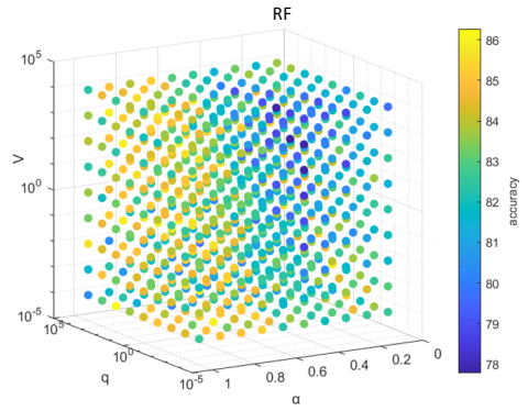
Figure 6. Knn algorithm success rates according to WCAR parameters
The WCAR method has three important parameters, which are V, q, and $\alpha$. According to the different values of these parameters, noise removal was performed from the Parkinson's walking signals. After cleaning, LBP classification processes were carried out with Knn, LR, and RF using the extracted features. The changes in the success rates according to these parameters are given in Figures 6, 7 and 8 for the three classification methods. Figures are shown in 4 dimensions. In order to understand whether it was successful, the transition of colors is checked in that the values are looked over to see for which parameters values they increase.
Figure 7. LR algorithm success rates according to WCAR parameters
Figure 8. RF algorithm success rates according to WCAR parameters
As mentioned earlier in the data set includes the entirety of three different studies. These studies are labeled as "Ga," "Ju," and "Si," and the performance values of all groups are given in Table 6. Success values were found separately for each group after the WCAR filter was applied. As seen in Table 6, the highest success in the data sets of "Ga" and "Ju" groups was found as 92.92% and 90.698%, respectively, with the Knn classifier. The most successful method was found in the "Si" group data set as 76.563% with RF.
Table 6. Success performances of data set groups
|
Data set |
Logistic Regression |
Knn |
Random Forest |
|
Ga |
79.646 |
92.920 |
89.38 |
|
Ju |
77.519 |
90.698 |
88.372 |
|
Si |
59.375 |
60.938 |
76.563 |
Walking signals were recorded from eight sensors connected to each foot. In order to indicate which foot signals were effective in diagnosing PD, the features extracted from said signals, which were recorded from the sensors on each foot, were subjected to the classification methods separately. The achieved success rates are given in Table 7.
Table 7. Success rates by feet
|
Filter Method |
Left foot |
Right Foot |
||||
|
LR |
RF |
Knn |
LR |
RF |
Knn |
|
|
CAR |
75.52 |
78.43 |
79.41 |
73.52 |
81.04 |
79.73 |
|
MCAR |
74.50 |
74.50 |
82.35 |
76.47 |
81.04 |
79.73 |
|
WCAR |
78.79 |
78.14 |
87.62 |
74.87 |
79.77 |
85.33 |
|
Without Filter |
76.14 |
73.85 |
81.69 |
76.14 |
74.50 |
80.06 |
When the success rates according to the feet are considered, the highest success rate was obtained with the features extracted as a result of the application of the WCAR filter method. Parkinson diagnosis was performed with a high success rate of 87.62% using Knn with the features extracted from the left foot sensors. It is gathered that more effective features were extracted from left foot sensors in general. When the features extracted after different filter methods and the extracted features without filter were examined, the features obtained from the left foot were found to be more successful than the right one. Knn was found to be more effective than other methods.
There are eight channels under each foot. In addition, there is a channel that shows the total force recorded from all channels. Each sensor measures signals from different parts of the foot soles. The success rates observed by using the extracted features after filter methods were applied to the signals recorded from each sensor are presented in Table 8. The classification process was carried out by RF.
Table 8. Success rates according to channels (For sensors on both feet)
|
Sensor |
CAR |
MCAR |
WCAR |
Without Filter |
|
Sensor 1 |
77.12 |
82.35 |
78.14 |
81.04 |
|
Sensor 2 |
78.43 |
79.08 |
77.49 |
74.18 |
|
Sensor 3 |
76.79 |
77.12 |
76.83 |
73.52 |
|
Sensor 4 |
75.16 |
74.50 |
78.79 |
75.16 |
|
Sensor 5 |
74.50 |
76.47 |
84.02 |
80.39 |
|
Sensor 6 |
75.16 |
72.22 |
75.85 |
77.45 |
|
Sensor 7 |
73.20 |
79.08 |
81.08 |
74.83 |
|
Sensor 8 |
76.79 |
72.22 |
80.75 |
77.45 |
|
Total force |
74.50 |
80.06 |
81.41 |
80.39 |
When the success rates according to the channels are considered, the highest success rate was observed with the signals recorded from Sensor 5. When looking at the filter methods, they were observed with the features extracted as a result of applying the WCAR filter method to the signals. The success rate was achieved as 84.02%. Sensor 4 is located right in the middle of the soles. Therefore, the signals obtained from the centers of the soles were shown to provide more effective signals compared to those in other areas.
After filter methods were applied to the signals recorded from the sensors, LBP transformation was applied, and then 12 statistical features were extracted from each sensor. In order to demonstrate the effectiveness of the features, classification processes were carried out using Knn according to each filter. The achieved success rates are given in Table 9.
Table 9. Success rates according to statistical features
|
Statistical Feature |
CAR |
MCAR |
WCAR |
Without Filter |
|
Mean |
63.07 |
63.07 |
67.35 |
60.45 |
|
Standard Deviation |
77.12 |
77.45 |
63.43 |
79.73 |
|
Energy |
76.47 |
74.18 |
83.04 |
80.06 |
|
Entropy |
79.41 |
79.08 |
85.33 |
76.47 |
|
Correlation |
81.69 |
80.06 |
84.98 |
70.58 |
|
Consecutive absolute differences |
72.87 |
71.89 |
79.12 |
79.41 |
|
Kurtosis |
71.89 |
72.54 |
81.41 |
59.47 |
|
Skewness |
80.06 |
82.02 |
85.62 |
75.81 |
|
Median |
80.39 |
82.02 |
85.94 |
76.14 |
|
Minimum |
81.37 |
69.93 |
71.60 |
59.15 |
|
Maximum |
77.45 |
79.08 |
84.35 |
81.37 |
|
Variance coefficient |
76.47 |
82.35 |
84.31 |
83.33 |
In Table 9, it is seen that the most successful of the extracted features after applying the CAR filter method to the signals is the minimum feature. After applying MCAR to the signals, the variation coefficient was seen to be the most successful feature. The median feature was seen as the most effective feature with WCAR, and without any filters, the most effective feature was the variation coefficient. The most successful feature was achieved by applying the WCAR filter method using the median attribute. In the most successful feature, a classification rate of 85.94% was observed.
Signals were recorded from 8 sensors beneath each person's foot and a channel displaying the total force of the signals recorded from these sensors. Features were extracted from 18 channels in total. Twelve statistical features were extracted from each channel. There are 18x12 = 216 features in total. It is known that not all features are effective in the diagnosis of PD. Features are reduced by the feature reduction method. The reduction was performed from the feature groups that were obtained according to different filter methods. Then the classification was done with Knn using the remaining features. The achieved success rates are given in Table 10.
Table 10. Success rates after feature reduction
|
Filter Method |
#Features |
LR |
Knn |
RF |
|
CAR |
18 |
82.12 |
86.79 |
88.75 |
|
MCAR |
29 |
84.41 |
88.66 |
87.37 |
|
WCAR |
30 |
86.43 |
92.96 |
89.96 |
|
Without Filter |
27 |
80.77 |
85.46 |
85.35 |
When Table 10 is considered, 18 features remained after applying the CAR filter method and reducing the removed features. After the classification, the highest success rate was observed with RF as 88.75%. After MCAR was applied, the highest success rate with 29 features was 88.66% with Knn; and after WCAR was applied, 30.9 attributes were used, and 92.96% success rate was observed with KNN. Without the filter, a success rate of 85.46% was achieved by using Knn with 27 features.
The approach proposed in this study was compared to other studies in the literature. Performance results of the studies performed on the same data set are given in Table 11. When Table 11 is considered, it was seen that the acceptable high success rates were obtained with the proposed approach.
Table 11. Comparison with the literature (%)
|
Author (s)/Year |
Features / Model |
Success Results |
All |
||
|
Ga |
Ju |
Si |
|||
|
Wu & Krishnan, 2009 [24] |
STC + LS-SVM / LOO Note: Part of the data set labeled as “Ju” was used |
- |
90.32 |
- |
- |
|
Lee and Lim, 2012 [20] |
WT+NEWFM |
- |
- |
- |
77.33 |
|
Zhang et al., 2013 [7] |
FT Coefficients + LC-KSVD |
|
|
|
83.44 |
|
Zhang et al., 2013 [7] |
FT Coefficients + SVM |
|
|
|
81.53 |
|
Daliri, 2013 [21] |
STFT + RBF kernel + SVM |
|
|
|
85.20 |
|
Daliri, 2013 [21] |
STFT+ Chi-square distance kernel+ SVM |
|
|
|
91.20 |
|
Khorasani and Daliri, 2014 [23] |
Stride time, swing time, stance time, double support time + HMM Note: Part of the data set labeled as “Ju” was used |
- |
90.3 |
- |
- |
|
Alkhatib et al. 2015 [18] |
Statistical + Knn |
83 |
- |
- |
- |
|
Perumal and Sankar, 2016 [1] |
Statistical (Step length, stride time, stance time, swing time, heel, below toe and toe forces and normalized heel, below toe and toe forces) + LDA |
92.25 |
92.5 |
90.0 |
- |
|
Alam et al., 2017 [5] |
VGRF statistics + SVM |
91.6 |
|
|
|
|
Alam et al., 2017 [5] |
SVM (Cubic) |
95.70 |
|
|
|
|
Ghaderyan & Fathi, 2021 [37] |
Inter-Limb Time-Varying Singular Value |
- |
- |
- |
95.59 |
|
El Maachi et al., 2020 [38] |
Deep 1d-Convnet |
- |
- |
- |
98.7 |
|
Yurdakul et al., 2020 [39] |
LBP+ ANN |
- |
- |
- |
98.3 |
|
This study |
[CAR, MCAR, WCAR]+LBP + Knn and LBP + RF |
92.92 |
90.698 |
76.563 |
92.96 |
In this study, a new approach was proposed to differentiate individuals with PD from healthy individuals through gait signals. Gait and tremor signals are widely used in the diagnosis of PD. Gait signals are generally measured in a multichannel way. While the signals are measured in one channel, other channels may encounter a noise effect. Therefore, CAR, MCAR, and WCAR methods were applied to the gait signals to remove possible noises in the signals. After applying the LBP conversion, statistical features were extracted from the formed clean signals. These feature groups were classified by classification algorithms such as Knn, LR, and RF. When the results are considered, it was determined that the WCAR method, which is an adaptive method, clears noise best. As the classification method, the best classifier was observed as the Knn method. The best success rate was found as 92.96%.
The study also examined signals on which foot was effective in diagnosing PD. According to the data set used, it was observed that the signals on the left foot provide better distinctive features in the diagnosis of PD. In addition, it was determined which sensors under the feet are effective in diagnosing PD.
In order to demonstrate the effectiveness of the proposed method, the classification process was performed by applying LBP transformation without applying noise-cleaning algorithms to the gait signals and by extracting statistical features. When the results were analyzed, it was determined that noise-cleaning methods increased overall success.
This study was performed in Siirt University Faculty of Engineering Machine Vision (MaVi) Laboratory. The authors of this article would like to thank the staff of MaVi Laboratory for their support.
[1] Perumal, S.V., Sankar, R. (2016). Gait and tremor assessment for patients with Parkinson’s disease using wearable sensors. ICT Express, 2(4): 168-174. https://doi.org/10.1016/j.icte.2016.10.005
[2] Morris, M.E., Huxham, F., McGinley, J., Dodd, K., Iansek, R. (2001). The biomechanics and motor control of gait in Parkinson disease. Clinical Biomechanics, 16(6): 459-470. https://doi.org/10.1016/S0268-0033(01)00035-3
[3] Lan, K.C., Shih, W.Y. (2014). Early Diagnosis of Parkinson's disease using a smartphone. Procedia Computer Science, 34: 305-312. https://doi.org/10.1016/j.procs.2014.07.028
[4] Abdulhay, E., Arunkumar, N., Narasimhan, K., Vellaiappan, E., Venkatraman, V. (2018). Gait and tremor investigation using machine learning techniques for the diagnosis of Parkinson disease. Future Generation Computer Systems, 83: 366-373. https://doi.org/10.1016/j.future.2018.02.009
[5] Alam, M.N., Garg, A., Munia, T.T.K., Fazel-Rezai, R., Tavakolian, K. (2017). Vertical ground reaction force marker for Parkinson’s disease. PLoS One, 12(5): e0175951. https://doi.org/10.1371/journal.pone.0175951
[6] Lai, D.T., Begg, R.K., Palaniswami, M. (2009). Computational intelligence in gait research: a perspective on current applications and future challenges. IEEE Transactions on Information Technology in Biomedicine, 13(5): 687-702. https://doi.org/10.1109/TITB.2009.2022913
[7] Zhang, Y., Ogunbona, P.O., Li, W., Munro, B., Wallace, G.G. (2013). Pathological gait detection of Parkinson's disease using sparse representation. In 2013 International Conference on Digital Image Computing: Techniques and Applications (DICTA), pp. 1-8. https://doi.org/10.1109/DICTA.2013.6691510
[8] Alkhatib, R., Corbier, C., El Badaoui, M., Moslem, B., Diab, M.O. (2015). Sensors' ground reaction force behavior for both normal and Parkinson subjects-a qualitative study. In 2015 37th Annual International Conference of the IEEE Engineering in Medicine and Biology Society (EMBC), pp. 4186-4189. https://doi.org/10.1109/EMBC.2015.7319317
[9] Tadano, S., Takeda, R., Miyagawa, H. (2013). Three dimensional gait analysis using wearable acceleration and gyro sensors based on quaternion calculations. Sensors, 13(7): 9321-9343. https://doi.org/10.3390/s130709321
[10] Muro-De-La-Herran, A., Garcia-Zapirain, B., Mendez-Zorrilla, A. (2014). Gait analysis methods: An overview of wearable and non-wearable systems, highlighting clinical applications. Sensors, 14(2): 3362-3394. https://doi.org/10.3390/s140203362
[11] Morris, M.E., McGinley, J., Huxham, F., Collier, J., Iansek, R. (1999). Constraints on the kinetic, kinematic and spatiotemporal parameters of gait in Parkinson's disease. Human Movement Science, 18(2-3): 461-483. https://doi.org/10.1016/S0167-9457(99)00020-2
[12] Whittle, M.W. (2014). Gait Analysis: An Introduction. Butterworth-Heinemann.
[13] Sarbaz, Y., Towhidkhah, F., Jafari, A., Gharibzadeh, S. (2012). Do the chaotic features of gait change in Parkinson's disease? Journal of Theoretical Biology, 307: 160-167. https://doi.org/10.1016/j.jtbi.2012.04.032
[14] Moore, S.T., MacDougall, H.G., Ondo, W.G. (2008). Ambulatory monitoring of freezing of gait in Parkinson's disease. Journal of Neuroscience Methods, 167(2): 340-348. https://doi.org/10.1016/j.jneumeth.2007.08.023
[15] Moore, S.T., MacDougall, H.G., Gracies, J.M., Cohen, H.S., Ondo, W.G. (2007). Long-term monitoring of gait in Parkinson's disease. Gait & Posture, 26(2): 200-207. https://doi.org/10.1016/j.gaitpost.2006.09.011
[16] Tripoliti, E.E., Tzallas, A.T., Tsipouras, M.G., Rigas, G., Bougia, P., Leontiou, M., Fotiadis, D.I. (2013). Automatic detection of freezing of gait events in patients with Parkinson's disease. Computer Methods and Programs in Biomedicine, 110(1): 12-26. https://doi.org/10.1016/j.cmpb.2012.10.016
[17] Camps, J., Sama, A., Martin, M., Rodriguez-Martin, D., Perez-Lopez, C., Arostegui, J.M.M., Rodriguez-Molinero, A. (2018). Deep learning for freezing of gait detection in Parkinson’s disease patients in their homes using a waist-worn inertial measurement unit. Knowledge-Based Systems, 139: 119-131. https://doi.org/10.1016/j.knosys.2017.10.017
[18] Alkhatib, R., Diad, M., Moslem, B., Corbier, C., El Badaoui, M. (2015). Gait-ground reaction force sensors selection based on ROC curve evaluation. Journal of Computer and Communications, 3(3): 13. https://doi.org/10.4236/jcc.2015.33003
[19] Samà, A., Pérez-López, C., Rodríguez-Martín, D., Català, A., Moreno-Aróstegui, J.M., Cabestany, J., Rodríguez-Molinero, A. (2017). Estimating bradykinesia severity in Parkinson's disease by analysing gait through a waist-worn sensor. Computers in Biology and Medicine, 84: 114-123. https://doi.org/10.1016/j.compbiomed.2017.03.020
[20] Lee, S.H., Lim, J.S. (2012). Parkinson’s disease classification using gait characteristics and wavelet-based feature extraction. Expert Systems with Applications, 39(8): 7338-7344. https://doi.org/10.1016/j.eswa.2012.01.084
[21] Daliri, M.R. (2013). Chi-square distance kernel of the gaits for the diagnosis of Parkinson's disease. Biomedical Signal Processing and Control, 8(1): 66-70. https://doi.org/10.1016/j.bspc.2012.04.007
[22] Zeng, W., Liu, F., Wang, Q., Wang, Y., Ma, L., Zhang, Y. (2016). Parkinson's disease classification using gait analysis via deterministic learning. Neuroscience Letters, 633: 268-278. https://doi.org/10.1016/j.neulet.2016.09.043
[23] Khorasani, A., Daliri, M.R. (2014). HMM for classification of Parkinson’s disease based on the raw gait data. Journal of Medical Systems, 38(12): 1-6. https://doi.org/10.1007/s10916-014-0147-5
[24] Wu, Y., Krishnan, S. (2009). Statistical analysis of gait rhythm in patients with Parkinson's disease. IEEE Transactions on Neural Systems and Rehabilitation Engineering, 18(2): 150-158. https://doi.org/10.1109/TNSRE.2009.2033062
[25] Yogev, G., Giladi, N., Peretz, C., Springer, S., Simon, E.S., Hausdorff, J.M. (2005). Dual tasking, gait rhythmicity, and Parkinson's disease: which aspects of gait are attention demanding? European Journal of Neuroscience, 22(5): 1248-1256. https://doi.org/10.1111/j.1460-9568.2005.04298.x
[26] Hausdorff, J.M., Lowenthal, J., Herman, T., Gruendlinger, L., Peretz, C., Giladi, N. (2007). Rhythmic auditory stimulation modulates gait variability in Parkinson's disease. European Journal of Neuroscience, 26(8): 2369-2375. https://doi.org/10.1111/j.1460-9568.2007.05810.x
[27] Frenkel‐Toledo, S., Giladi, N., Peretz, C., Herman, T., Gruendlinger, L., Hausdorff, J.M. (2005). Treadmill walking as an external pacemaker to improve gait rhythm and stability in Parkinson's disease. Movement disorders: official journal of the Movement Disorder Society, 20(9): 1109-1114. https://doi.org/10.1002/mds.20507
[28] Frenkel-Toledo, S., Giladi, N., Peretz, C., Herman, T., Gruendlinger, L., Hausdorff, J.M. (2005). Effect of gait speed on gait rhythmicity in Parkinson's disease: variability of stride time and swing time respond differently. Journal of Neuroengineering and Rehabilitation, 2(1): 1-7. https://doi.org/10.1186/1743-0003-2-23
[29] Goldberger, A.L., Amaral, L.A., Glass, L., Hausdorff, J.M., Ivanov, P.C., Mark, R.G., Stanley, H.E. (2000). PhysioBank, PhysioToolkit, and PhysioNet: Components of a new research resource for complex physiologic signals. Circulation, 101(23): e215-e220. https://doi.org/10.1161/01.CIR.101.23.e215
[30] http://physionet.org, “Gait in Parkinson’s Disease,” last access June 25, 2021.
[31] Kaya, Y., Uyar, M., Tekin, R., Yıldırım, S. (2014). 1D-local binary pattern based feature extraction for classification of epileptic EEG signals. Applied Mathematics and Computation, 243: 209-219. https://doi.org/10.1016/j.amc.2014.05.128
[32] Kuncan, F., Kaya, Y., Kuncan, M. (2019). New approaches based on local binary patterns for gender identification from sensor signals. J Fac Eng Archit Gazi Univ, 34(4): 2173-2185. https://doi.org/10.17341/gazimmfd.426259
[33] Kuncan, F., Kaya, Y., Kuncan, M. (2019). A novel approach for activity recognition with the down-sampling 1D local binary pattern. Advances in Electrical and Computer Engineering, 19(1): 35-44.
[34] Rousseeuw, P.J., Hubert, M. (2011). Robust statistics for outlier detection. Wiley Interdisciplinary Reviews: Data Mining and Knowledge Discovery, 1(1): 73-79. https://doi.org/10.1002/widm.2
[35] Khorasani, A., Shalchyan, V., Daliri, M.R. (2019). Adaptive artifact removal from intracortical channels for accurate decoding of a force signal in freely moving rats. Frontiers in Neuroscience, 13: 350. https://doi.org/10.3389/fnins.2019.00350
[36] Ertuğrul, Ö.F., Kaya, Y., Tekin, R., Almalı, M.N. (2016). Detection of Parkinson's disease by shifted one dimensional local binary patterns from gait. Expert Systems with Applications, 56: 156-163. https://doi.org/10.1016/j.eswa.2016.03.018
[37] Ghaderyan, P., Fathi, G. (2021). Inter-limb time-varying singular value: A new gait feature for Parkinson’s disease detection and stage classification. Measurement, 177: 109249. https://doi.org/10.1016/j.measurement.2021.109249
[38] El Maachi, I., Bilodeau, G.A., Bouachir, W. (2020). Deep 1D-convnet for accurate Parkinson disease detection and severity prediction from gait. Expert Systems with Applications, 143: 113075. https://doi.org/10.1016/j.eswa.2019.113075
[39] Yurdakul, O.C., Subathra, M.S.P., George, S.T. (2020). Detection of Parkinson’s disease from gait using neighborhood representation local binary patterns. Biomedical Signal Processing and Control, 62: 102070. https://doi.org/10.1016/j.bspc.2020.102070