Ji Zou | Chao Zhang | Zhongjing Ma*
© 2021 IIETA. This article is published by IIETA and is licensed under the CC BY 4.0 license (http://creativecommons.org/licenses/by/4.0/).
OPEN ACCESS
Human structure-based plantar pressure (PP) analysis has been widely used in medical, sports, footwear design, and footwear sales. The current studies mostly focus on the development of PP measuring technologies and the analysis of pressure distribution features based on sensing results. Relatively few scholars have tried to analyze PP through image processing. To bridge the gap, this paper tries to classify PP images based on convolutional neural network (CNN). Firstly, the authors prepared the zoning and center calculation for PP images, and established a PP image classification model. Then, the PP image features were selected dynamically based on sparse, low-redundancy feature subsets, and the results of principal component analysis (PCA) were combined with the CNN to realize dynamic extraction of features from PP images. Finally, an image classification algorithm was designed based on the inter-area difference in PP distribution. The proposed algorithm was proved feasible through experiments. The research findings provide a reference for processing pressure images in other scenarios.
plantar pressure (PP) analysis, convolutional neural network (CNN), feature selection, feature extraction
Human structure-based plantar pressure (PP) analysis has been widely applied. In the medical field, plantar features are used to assess whether the bones are healthy, and assist with the doctors in diagnosing the patients with foot disease or those having trouble walking due to brain disease [1-4]. In the field of sports, more and more researchers have paid attention to the variation in PP distribution induced by the changing sports pattern [5-7]. PP measurement and analysis are also meaningful in the design and purchase of sneakers [8-10].
In health monitoring and medical diagnosis, the existing detection devices for PP distribution are very expensive and not portable [11-16]. Sathish Babu et al. [17] designed a PP distribution measuring insole with conductive fabric and the microporous filter membrane, and optimized the sensitivity and response time of the device by regulating the ion liquid load; the authors analyzed the PP distribution features under different poses, identified the pressure center, and examined the proportion of the main bearing area and variation of PP; on this basis, the gait process was calibrated according to the analysis results.
When the pressure measuring insole moves, the PP measurement system often has a large error due to signal attenuation [18-22]. Through thorough consideration of multiple attributes of flexible sensing materials, Neri et al. [23] designed the framework for a system based on multiplexing circuit with a resistive voltage amplifier and Ardunio module, and chose Windows Forms (WinForms) and MongoDB to realize software visualization and data storage, respectively.
There are two common human gait analysis methods. One is optical image acquisition, which has a high cost and a high recognition rate. The other is sensor acquisition, which offers a variety of optional sensors. Anzai et al. [24] collected PP and foot pose information with a sensor array, reduced the dimensionality and noise level of the collected data through singular value decomposition (SVD) and principal component analysis (PCA), and established a pose-based gait model to correct the error of kinematical modeling, which arises from the omission of foot movement. Castro et al. [25] analyzed the PP features of flatfeet based on the PP distribution images of youngsters, and drew two important conclusions through contrastive experiments: the flatfoot group had a much higher momentum in different areas of the foot than the normal foot group, and the pressure trajectory at the pressure center skewed outside among the flatfeet subjects. Sadler et al. [26] collected the PP distribution images of multiple modes of motions, namely, walking, running, ascending steps, and descending steps, divided the PP areas in the images into eight regular arrays, constructed a solving equation for the point of action for the resultant ground reaction force to the planar under the multi-motion model, and obtained the influence law of the peak force in different plantar bearing areas on the plantar force. Aqueveque et al. [27] predicted the PP distribution by least mean squares (LMS) and recursive least squares (RLS) adaptive filtering algorithms, analyzed the coefficients and monotonicity of PP distribution features and joint angles, divided the gait cycle of subjects based on the analysis results, and further classified the PP images through gait recognition.
The current studies mostly focus on the development of PP measuring technologies and the analysis of pressure distribution features based on sensing results. Relatively few scholars have tried to analyze PP through image processing. This paper attempts to classify PP images based on convolutional neural network (CNN). Section 2 summarizes the workflow of PP image classification; Section 3 presents the zoning and center calculation methods for PP images; Section 4 builds up a classification model for PP images; Section 5 dynamically selects the features of PP images based on sparse, low-redundancy feature subsets, and reduces the complexity of CNN feature extraction by combing the PCA results with the CNN. Section 6 puts forward an image classification algorithm based on the inter-area difference in PP distribution. The proposed algorithm was proved feasible through experiments
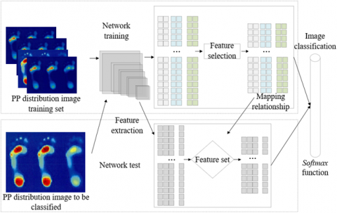
Figure 1. Flow chart of CNN-based PP image classification algorithm
Figure 1 shows the workflow of the CNN-based PP image classification algorithm. By zoning and computing the center of PP images, the algorithm extracts the difference of PP distributions in different areas. Then, the CNN is combined with PP area feature selection algorithm to dynamically describe PP image feature distribution by Gaussian mixture model and classify the images based on inter-area distribution difference.
Figure 2. Dynamic acquisition of PP image data
The PP center can effectively represent the direction of PP. The ground reaction force at this point is equivalent to the resultant force of the ground reaction forces acting on different areas of the planta. Figure 2 gives an example of the dynamic acquisition of PP image data. Let MC and MR be the number of columns and rows in the established static PP matrix, respectively; Wij be the pressure. Then, the abscissa and ordinate of PP center to be solved can be respectively expressed as:
${{O}_{a}}=\sum\limits_{i=1}^{{{M}_{C}}}{\sum\limits_{j=1}^{{{M}_{R}}}{i\times {{W}_{ij}}/}}\sum\limits_{i=1}^{{{M}_{C}}}{\sum\limits_{j=1}^{{{M}_{R}}}{{{W}_{ij}}}}$ (1)
${{O}_{b}}=\sum\limits_{j=1}^{{{M}_{R}}}{\sum\limits_{i=1}^{{{M}_{C}}}{j\times {{W}_{ij}}/}}\sum\limits_{i=1}^{{{M}_{C}}}{\sum\limits_{j=1}^{{{M}_{R}}}{{{W}_{ij}}}}$ (2)
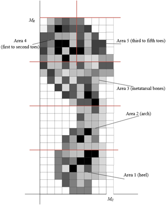
Figure 3. Dynamic zoning of PP image
Similarly, the ground reaction force at the local pressure center is equivalent to the resultant force of the ground reaction forces acting on the local plantar area. Here, the planta is divided into five areas with independent pressure centers. The dynamic zoning of PP image is illustrated in Figure 3. The abscissa Ia1 and ordinate Ib1 of the pressure center of local area 1 can be respectively calculated by:
${{I}_{a\text{1}}}=\sum\limits_{i=1}^{{{M}_{C}}}{\sum\limits_{j=1}^{{{M}_{R}}/4}{i\times {{W}_{ij}}/}}\sum\limits_{i=1}^{{{M}_{C}}}{\sum\limits_{j=1}^{{{M}_{R}}/4}{{{W}_{ij}}}}$ (3)
${{I}_{b\text{1}}}=\sum\limits_{j=1}^{{{M}_{R}}/4}{\sum\limits_{i=1}^{{{M}_{C}}}{j\times {{W}_{ij}}/}}\sum\limits_{i=1}^{{{M}_{C}}}{\sum\limits_{j=1}^{{{M}_{R}}/4}{{{W}_{ij}}}}$ (4)
The abscissa Ia2 and ordinate Ib2 of the pressure center of local area 1 can be respectively calculated by:
${{I}_{a\text{2}}}=\sum\limits_{i=1}^{{{M}_{C}}}{\sum\limits_{j={{M}_{R}}/4}^{{{M}_{R}}/2}{i\times {{W}_{ij}}/}}\sum\limits_{i=1}^{{{M}_{C}}}{\sum\limits_{j={{M}_{R}}/4}^{{{M}_{R}}/2}{{{W}_{ij}}}}$ (5)
${{I}_{b\text{2}}}=\sum\limits_{j={{M}_{R}}/4}^{{{M}_{R}}/2}{\sum\limits_{i=1}^{{{M}_{C}}}{j\times {{W}_{ij}}/}}\sum\limits_{i=1}^{{{M}_{C}}}{\sum\limits_{j={{M}_{R}}/4}^{{{M}_{R}}/2}{{{W}_{ij}}}}$ (6)
The abscissa Ia3 and ordinate Ib3 of the pressure center of
local area 3 can be respectively calculated by:
${{I}_{a\text{3}}}=\sum\limits_{i=1}^{{{M}_{C}}}{\sum\limits_{j={{M}_{R}}\text{/}2}^{\text{3}{{M}_{R}}\text{/}\mathbf{4}}{i\times {{W}_{ij}}/}}\sum\limits_{i=1}^{{{M}_{C}}}{\sum\limits_{j={{M}_{R}}\text{/}2}^{\text{3}{{M}_{R}}\text{/}\mathbf{4}}{{{W}_{ij}}}}$ (7)
${{I}_{b\text{3}}}=\sum\limits_{j={{M}_{R}}\text{/}2}^{\text{3}{{M}_{R}}\text{/}4}{\sum\limits_{i=1}^{{{M}_{C}}}{j\times {{W}_{ij}}/}}\sum\limits_{i=1}^{{{M}_{C}}}{\sum\limits_{j={{M}_{R}}\text{/}2}^{\text{3}{{M}_{R}}\text{/}\mathbf{4}}{{{W}_{ij}}}}$ (8)
The abscissa Ia4 and ordinate Ib4 of the pressure center of local area 4 can be respectively calculated by:
${{I}_{a\text{4}}}=\sum\limits_{i=1}^{{{M}_{C}}/2}{\sum\limits_{j=\text{3}{{M}_{R}}\text{/}4}^{{{M}_{R}}}{i\times {{W}_{ij}}/}}\sum\limits_{i=1}^{{{M}_{C}}/2}{\sum\limits_{j=\text{3}{{M}_{R}}\text{/}4}^{{{M}_{R}}}{{{W}_{ij}}}}$ (9)
${{I}_{b\text{4}}}=\sum\limits_{j=\text{3}{{M}_{R}}\text{/}4}^{{{M}_{R}}}{\sum\limits_{i=1}^{{{M}_{C}}/2}{j\times {{W}_{ij}}/}}\sum\limits_{i=1}^{{{M}_{C}}/2}{\sum\limits_{j=\text{3}{{M}_{R}}\text{/}4}^{{{M}_{R}}}{{{W}_{ij}}}}$ (10)
The abscissa Ia5 and ordinate Ib5 of the pressure center of local area 5 can be respectively calculated by:
${{I}_{a\text{5}}}=\sum\limits_{i={{M}_{C}}/2}^{{{M}_{C}}}{\sum\limits_{j=\text{3}{{M}_{R}}\text{/}4}^{{{M}_{R}}}{i\times {{W}_{ij}}/}}\sum\limits_{i={{M}_{C}}/2}^{{{M}_{C}}}{\sum\limits_{j=\text{3}{{M}_{R}}\text{/}4}^{{{M}_{R}}}{{{W}_{ij}}}}$ (11)
${{I}_{b\text{4}}}=\sum\limits_{j=\text{3}{{M}_{R}}\text{/}4}^{{{M}_{R}}}{\sum\limits_{i={{M}_{C}}/2}^{{{M}_{C}}}{j\times {{W}_{ij}}/}}\sum\limits_{i={{M}_{C}}/2}^{{{M}_{C}}}{\sum\limits_{j=\text{3}{{M}_{R}}\text{/}4}^{{{M}_{R}}}{{{W}_{ij}}}}$ (12)
This paper proposes an image processing method for feature selection from PP areas, with the goal to dynamically extract the difference of PP distribution features in different areas from PP images. The CNN was combined with PP area feature selection algorithm. The former was used to dynamically extract image features for PP image training set, and the latter was used to select features that contribute greatly to classification for image classification. Figure 4 displays the workflow of the image classification method for PP area feature selection.
Figure 4. Image classification method for PP area feature selection
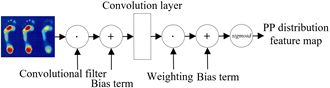
In the established CNN, the convolution kernel is 3 pixels in height and 3 pixels in width. Through max pooling, the pooling layer reduces the dimensionality and size of the target PP image, and extracts the PP features from that image. Then, the fully connected layer, which contains at least one hidden layer, fuses the PP local features into global features of PP. Figure 5 explains the convolution and feature extraction process of the CNN. Let g be the activation function; spz be the bias term; ωpz be the connection weight between neurons of different layers; IVr and MT be the r-th feature and total number of features of the input vector, respectively. Then, the neurons σpz on the q-th layer of the CNN can be calculated by:
${{g}_{{{\sigma }_{pz}}}}=g\left( {{s}_{pz}}+\sum\limits_{r=1}^{{{M}_{T}}}{{{\omega }_{pz}}\times I{{V}_{r}}} \right)$ (13)
Figure 5. Flow chart of convolution and feature extraction of the CNN
This paper dynamically selects PP image features, using sparse, low-redundancy feature subsets. The algorithm first dynamically acquires the cluster distribution of the original PP image sample in the space by spectral clustering. Let B be the class label of each local area in the PP image; ω be the weight matrix for selecting PP features embedded in local areas; ξ(B) be the score of the clustering results on the previous spectrum, which covers angle cosine similarity and contour coefficient; Φ(ω) be the regularization term maintaining the sparsity and low-redundancy of the feature; β and γ be the weight parameter of the loss function and Φ(ω) coefficient, respectively. Then, the selection of embedded local PP features can be converted into a constrained optimization problem, whose objective function and constraint can be respectively described as:
$\begin{align} & minK\left( B,\omega \right)=\underset{B,\omega }{\mathop{min}}\,\xi \left( B \right)+\beta \left[ k\left( B,\omega A \right)+\gamma \Phi \left( \omega \right) \right] \\ & S.T. B\ge 0,\omega \ge 0 \\\end{align}$ (14)
Under the constraints of the non-negativity of B and ω, the loss function can be expressed as:
$k\left( B,\omega A \right)=\left\| A\omega -B \right\|_{2}^{2}$ (15)
Let T(*) be the trace of matrix. Then, Φ(ω) can be described as:
$\Phi \left( \omega \right)=\frac{1}{2}\left( {{\left\| \omega {{\omega }^{T}} \right\|}_{1}}-T\left( \omega {{\omega }^{T}} \right) \right)$ (16)
The trace norm can be simplified as:
$\Phi \left( \omega \right)=\frac{1}{2}\left( {{\left\| \omega {{\omega }^{T}} \right\|}_{1}}-\left\| \omega {{\omega }^{T}} \right\|_{2}^{2} \right)$ (17)
Combining formulas (15), (17), and (14):
$\begin{align} & minK\left( B,\omega \right)=\underset{B,\omega }{\mathop{min}}\,\xi \left( B \right) \\ & +\beta \left[ \left\| A\omega -B \right\|_{2}^{2}+\frac{\gamma }{2}\left( {{\left\| \omega {{\omega }^{T}} \right\|}_{1}}-\left\| \omega {{\omega }^{T}} \right\|_{2}^{2} \right) \right] \\ & S.T. B\ge 0,\omega \ge 0 \\\end{align}$ (18)
After solving the constrained optimization of regional PP feature selection, the algorithm will output the final selected PP features of the area, that is, the PP features in the area with relatively large weight.
Once the features are selected, the matrix can be transformed to map high-dimensional features to low-dimensional features. Here, the PCA is integrated with the CNN to realize feature extraction, by replacing the original PP image features with a few potential features. The PCA aims to find a hyperplane that is as close to each sample in the low-dimensional space as possible, which supports one-to-one mapping to the high-dimensional space. Let A={a1, a2, …, aMT} be the PP image sample set; ∑ai=0 be the centralization of the samples; Q={θ1, θ2, …, θi…, θc} be a new coordinate system, with θi be the standard orthogonal basis vector. Then, the hyperplane must be constrained by:
${{\left\| {{\theta }_{i}} \right\|}_{2}}=1,\theta _{i}^{T}{{\theta }_{j}}=0$ (19)
The mapping of local PP image sample ai in the low-dimensional space can be expressed as fi=(fi1, fi2, …, fij, …, fic), where fij=θTjai is the j-th dimensional feature of ai in the low-dimensional space. In the low-dimensional space, the original PP sample can be reconstructed from the hyperplane:
$a_{i}^{*}=\sum\limits_{j=1}^{c}{{{f}_{ij}}{{\theta }_{j}}}$ (20)
For the local PP image sample set in the high-dimensional space, the difference between each original image and the reconstructed image can be represented by their distance. The optimization objective that the hyperplane should remain close to each sample can be expressed as:
$min\sum\limits_{i=1}^{{{M}_{T}}}{\left\| \sum\limits_{j=1}^{c}{{{f}_{ij}}{{\theta }_{j}}-{{a}_{i}}} \right\|}_{2}^{2}$ (21)
The above formula can be simplified as:
$\min _{\omega}-T\left(Q^{T} A A^{T} Q\right)$
S.T. $\quad Q^{T} Q=\mathrm{I}$ (22)
To ensure that the local PP image samples in low-dimensional space have a sufficiently large distribution variance, another optimization objective should be defined: the sample projections on the hyperplane should be separated as much as possible. The distribution variance can be expressed as:
$\sum\limits_{i}{{{Q}^{T}}{{a}_{i}}a_{i}^{T}Q}$ (23)
The corresponding optimization objective can be expressed as:
$\max _{\omega}-T\left(Q^{T} A A^{T} Q\right)$
S.T. $\quad Q^{T} Q=\mathrm{I}$ (24)
When the above two constraints are satisfied at the same time, the PP images can be subjected to the PCA.
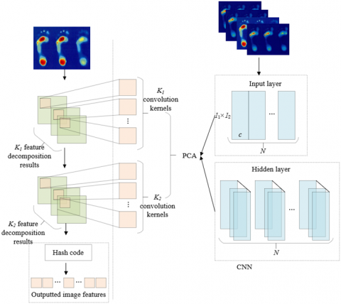
Figure 6. Structure of composite model
This paper integrates the PCA results with the CNN to effectively reduce the computing complexity of the latter. The composite model structure is shown in Figure 6. The input layer of the CNN completes the samples of PP distribution features. Based on the zoning of PP images (each area has an independent pressure center), the size of the l-th area is defined as l1*l2. Then, the pixel matrix of each area was converted into a column vector. After that, all column vectors were combined into the feature matrix of the entire image. Let ai be the feature matrix of the i-th image. Since each image is divided into 5 areas, the full feature matrix contains 5 columns. Then, the full feature matrix corresponding to the PP image sample set containing N training samples can be expressed as:
$A=\left[ {{A}_{1}},{{A}_{2}},...,{{A}_{N}} \right]\in {{\Re }^{{{l}_{1}}{{l}_{2}}\times 5N}}$ (25)
The AAT eigenvalue decomposition results obtained through the PCA were sorted in descending order. The first K1 terms were selected to form an l1×l2 matrix:
$Q_{k}^{1}=ma{{t}_{{{l}_{1}},{{l}_{2}}}}\left( {{r}_{k}}\left( A{{A}^{T}} \right) \right)\in {{\Re }^{{{l}_{1}}\times {{l}_{2}}}}$ (26)
In the input layer of the CNN, the original image features are extracted by K1 channels, i.e., convolution kernels. The local PP image features received by the second layer of the CNN can be described as the following matrix:
$B=\left[ {{B}^{1}},{{B}^{2}},...,{{B}^{{{K}_{2}}}} \right]\in {{\Re }^{{{l}_{1}}{{l}_{2}}\times 5{{K}_{1}}}}$ (27)
Then, the BBT eigenvalue decomposition results obtained by the PCA were sorted in descending order. The first K2 terms were selected to form a convolution kernel:
$Q_{{{N}_{S}}}^{2}=MA{{T}_{{{l}_{1}},{{l}_{2}}}}\left( {{r}_{{{N}_{S}}}}\left( B{{B}^{T}} \right) \right)\in {{\Re }^{{{l}_{1}}\times {{l}_{2}}}}$ (28)
The final image features that meet the task requirements can be obtained through the histogram processing at the output of the first layer of the CNN, the binarization at the output of the second layer, and hash coding. The CNN generates the convolution kernel based on PCA results, providing a benchmark for the dimensionality reduction algorithm of feature extraction.
Our algorithm, responsible for selecting the features representing the inter-area difference in PP distribution, can be divided into two parts: the feature distribution description based on Gaussian mixture model, and the detection of inter-area distribution difference. Let ε and λ be the standard error and mean of the probability density function (PDF) W(a) of Gaussian mixture model, respectively. Then, the PDF can be defined as:
$W\left( a \right)=\frac{1}{\sqrt{2\pi {{\varepsilon }^{2}}}}{{e}^{\frac{-{{\left( a-\lambda \right)}^{2}}}{2{{\varepsilon }^{2}}}}}$ (29)
After fully considering the class labels of each local area of a PP image sample, the Gaussian mixture model could be adopted to illustrate the regional pressure distribution of each dimensional features of the PP image. The inter-area difference can be measured by the indices designed for model parameters.
Suppose the convolution and pooling layers of the CNN extract n features from the PP image sample. Then, the feature matrix composed of the n features is the input of the feature selection algorithm. Then, the set of the σ-dimensional features of the image sample can be denoted as Aσ={aσ1, aσ2, …, aσMS}, where σ=1, 2, …n, and the number of image samples can be denoted as MS. According to the class label B of each local area, the subset of each d-dimensional feature can be generated as:
${{A}_{\sigma }}=A_{\sigma }^{\left( 1 \right)}\cup A_{\sigma }^{\left( 2 \right)}\cup ...\cup A_{\sigma }^{\left( t \right)}\cup ...\cup A_{\sigma }^{\left( {{N}_{B}} \right)}$ (30)
where, B=1, 2, …NB. The eigenvalues of the σ-dimensional image samples belonging to class B can be represented as A(B)σ.
To measure the PP distribution difference between A(1)σ,A(2)σ,…,A(τ)σ,…,A(NB)σ, the distribution of A(B)σ can be described by the Gaussian mixture model. Suppose there are a total of L Gaussian functions, and the weight of the i-th function is δi, satisfying ∑Li=1δi=1. Let λi and εi be the mean and standard error of δi, respectively. Referring to formula (29), the Gaussian mixture model WH(a) can be defined as:
${{W}_{H}}\left( a \right)=\sum\limits_{i=1}^{L}{{{\delta }_{i}}W\left( a|{{\lambda }_{i}},{{\varepsilon }_{i}} \right)}$ (31)
Although WH(a) has relatively few parameters, the derivation of the objective function is a rather complex process. Based on maximum likelihood estimation, this paper solves and optimizes δi, λi, and εi. That is, the probabilities of local PP distribution image samples to fall in a class obey the Gaussian distribution in the iterative process. Let MB be the number of samples in A(B)σ. Then, the optimization objective of WH(a) can be given by:
$maxlnK\left( A_{\sigma }^{\left( B \right)} \right)=ln\left( \underset{j=1}{\overset{{{M}_{B}}}{\mathop{\prod }}}\,{{W}_{H}}\left( {{a}_{\sigma j}} \right) \right),{{a}_{\sigma j}}\in A_{\sigma }^{\left( B \right)}$ (32)
Combining formula (32) with formula (31):
$maxlnK\left( A_{\sigma }^{\left( B \right)} \right)=\sum\limits_{j=1}^{{{M}_{B}}}{ln\left( \sum\limits_{i=1}^{L}{{{\delta }_{i}}\cdot W\left( {{a}_{\sigma j}}|{{\lambda }_{i}},{{\varepsilon }_{i}} \right)} \right)}$ (33)
The above formula (33) can be solved iteratively with the expectation-maximization (EM) algorithm. Dividing A(B)σ by the current WH(a), the Gaussian mixture components of eigenvalue aσi can be described by uj ∈{1, 2, …L}. Since the classification criterion is to check whether the mixture components take up the largest proportion, the posterior probability of uj can be expressed as:
${{W}_{H}}\left( {{u}_{j}}=i|{{a}_{\sigma j}} \right)=\frac{W\left( {{u}_{j}}=i \right)\cdot {{W}_{H}}\left( {{a}_{\sigma j}}|{{c}_{j}}=i \right)}{{{W}_{H}}\left( {{a}_{\sigma j}} \right)}$ (34)
The division results μi of A(B)σ can be described as:
${{\mu }_{j}}=\underset{i\in \left\{ 1,2,...,l \right\}}{\mathop{argmax}}\,{{W}_{H}}\left( {{u}_{j}}=i|{{a}_{\sigma j}} \right)$ (35)
Let MB-I be the number of local PP distribution images that provide the features to the i-th Gaussian function. According to the current division results, the model parameters δi, λi, and εi can be respectively updated by:
${{\delta }_{i}}=\frac{1}{{{M}_{B-i}}}\sum\limits_{j=1}^{{{M}_{B-i}}}{{{W}_{H}}\left( {{u}_{j}}=i|{{a}_{\sigma j}} \right)}$ (36)
${{\lambda }_{i}}=\frac{\sum\limits_{j=1}^{{{M}_{B-i}}}{{{W}_{H}}\left( {{u}_{j}}=i|{{a}_{\sigma j}} \right){{a}_{\sigma j}}}}{\sum\limits_{j=1}^{{{M}_{B-i}}}{{{W}_{H}}\left( {{u}_{j}}=i|{{a}_{\sigma j}} \right)}}$ (37)
${{\varepsilon }_{i}}=\frac{\sum\limits_{j=1}^{{{M}_{B-i}}}{{{W}_{H}}\left( {{u}_{j}}=i|{{a}_{\sigma j}} \right){{\left( {{a}_{\sigma j}}-{{\lambda }_{i}} \right)}^{2}}}}{\sum\limits_{j=1}^{{{M}_{B-i}}}{{{W}_{H}}\left( {{u}_{j}}=i|{{a}_{\sigma j}} \right)}}$ (38)
Figure 7 presents the distribution of features with the same inter-area difference. Let λi and δi denote the position and the class weight of position feature of the i-th Gaussian function, respectively. When the L is fixed, the inter-area difference in PP image feature distribution can be measured by adjusting δi, λi, and εi. The difference Dσ of Aσ can be calculated by:
${{D}_{\sigma }}=max\left\{ {{\left\| D_{\sigma }^{\left( 1 \right)} \right\|}_{\infty }},{{\left\| D_{\sigma }^{\left( 2 \right)} \right\|}_{\infty }},...,{{\left\| D_{\sigma }^{\left( \tau \right)} \right\|}_{\infty }},...,{{\left\| D_{\sigma }^{\left( {{N}_{B}} \right)} \right\|}_{\infty }} \right\}$ (39)
Figure 7. Distribution of features with the same inter-area difference
Each class of features correspond to a Gaussian mixture model, which contains a vector composed of the differences between the L functions. Let Q(B)σ=[d(B)σ1,d(B)σ2,…d(B)σi,…,d(B)σL]T be the difference vector of Class B features; λ' and ε' be the mean and standard error of the Gaussian mixture model the closest to the λi, as measured by Gaussian distance, respectively. Then, the q(τ)σi in Q(B)σ can be measured by:
$q_{\sigma i}^{\left( B \right)}={{\delta }_{i}}\times \left| {{\lambda }_{i}}-{\lambda }' \right|\times {{d}^{-max\left( {{\varepsilon }_{i}},{\varepsilon }' \right)}}$ (40)
Formula (40) shows the difference between λi and λ', the difference between εi and ε', and δi are all positively correlated with q(B)σi.
Table 1. Pressure distribution in each area of the planta
|
|
Area 1 |
Area 2 |
Area 3 |
Area 4 |
Area 5 |
|
Static pressure |
56.32 |
15.09 |
55.72 |
19.75 |
17.35 |
|
Peak pressure |
73.95 |
19.72 |
62.34 |
20.53 |
19.59 |
|
Proportion |
30.21 |
13.76 |
30.31 |
14.12 |
16.6 |
This paper divides the planta into five areas: Area 1 (heel), Area 2 (arch), Area 3 (metatarsal bones), Area 4 (first to second toes), and Area 5 (third to fifth toes). Table 1 shows the test results on the PP in each area of a subject. It can be seen that the two peaks of PP existed in Area 1 and Area 3, which together accounted for more than 65% of the total PP. Areas 2-5 were under relatively small pressure. Among them, Area 2 faced the least pressure.
Figure 8 provides the relationship curve between PP center position and pressure. It can be inferred that the peak pressures (741N at the maximum) appeared at the PP center of planta (0mm, and 100mm) and that of metatarsal bones (240mm, and 300mm). The results are consistent with the pressure distribution in Table 1.
Figure 8. Relationship between PP center position and pressure
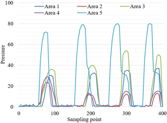
Figure 9. Dynamic PP change curves in different areas
Figure 9 records the dynamic PP change curves in different areas. These curves reflect the good gait features of a subject during normal walking. The PP data are not greatly disturbed by noise, and can serve as the reference data for PP analysis and classification.
Figure 10 displays the force on each area of left and right feet under different gait cycles. The mean peak pressures of the five plantar areas correspond to the gait phases of the subject. It can be learned that a gait cycle can be divided into a double support phase where both feet are on the ground, and a swing phase where only one foot is on the ground. The first phase takes up 59% of the cycle, and the second, 41%. Based on the PP images of the two feet, it is possible to determine to which phase the subject belongs. As shown in Figure 10, the minimum and maximum peak pressures of the two feet both appeared in the double support phase. Whether the subject belongs to the double support phase can be judged by the peak pressures on Areas 1 and 3.
Figure 10. Force on each area of left and right feet under different gait cycles
Table 2. Classification results on different types of planta
|
|
Left foot |
Right foot |
Proportion of correct recognitions |
Classification accuracy |
|
Inclined |
30/30 |
29/30 |
29/30 |
96.7% |
|
Broken |
30/30 |
30/30 |
30/30 |
100% |
|
Mixed |
30/30 |
30/30 |
30/30 |
100% |
|
Normal |
89/90 |
87/90 |
86/90 |
95.6% |
Table 3. Recognition effects of different methods
|
|
Left foot |
Right foot |
Proportion of correct recognitions |
Classification accuracy |
|
Edge distance |
69/70 |
68/70 |
67/70 |
95.7% |
|
Spectrum feature |
67/70 |
68/70 |
65/70 |
92.9% |
|
Spectrum feature + regional pressure |
65/70 |
69/70 |
64/70 |
91.4% |
|
Our method |
69/70 |
69/70 |
68/70 |
97.1% |
Figure 11. Time cost of each stage of model training and test
The proposed PP image classification model was trained with and used to recognize four different types of PP distribution images: inclined, broken, mixed, and normal. The classification accuracy of each type is listed in Table 2. Obviously, our model achieved very high recognition rates and classification accuracies on the three abnormal planta (inclined, broken, and mixed). The good performance is attributable to two factors: First, the zoning of planta helps to extract the key features from local PP distribution images, and simplify image preprocessing. Second, the feature selection and extraction avoid the arch area, but focus on Areas 1 and 3, where the pressure changes insignificantly; this contributes to the good classification effect on special planta that are inclined or broken.
Observations show that the PP images had smaller shape change than the PP distribution data, in which every frame was constantly changing. This also manifests that our classification strategy, which is based on inter-area distribution difference, is highly scientific. To further verify its effectiveness, our PP image classification method was compared with three common PP recognition approaches (Table 3).
Finally, the time cost of our PP image classification model in each stage of network training and test was counted to demonstrate the practicality of the model. As shown in Figure 11, our model needs to spend extra time in feature selection during network training and in classifier reconstruction during network test, because feature selection and classifier reconstruction are introduced to the traditional CNN. However, the time costs of the two parts only accounted for 2% of all the time consumed. This means the additional links of our model do not greatly affect the time cost. In fact, these links make our model more practical, while ensuring the classification effect.
This paper envisages a PP image classification method based on the CNN. Firstly, the authors introduced the strategies for zoning and center calculation for PP images, constructed a PP image classification model, and provided the methods for PP feature selection and extraction. After that, an image classification algorithm was developed based on the inter-area PP distribution difference. In addition, the authors plotted the relationship between PP center position and pressure, and the dynamic changes of PP in different areas, providing valuable reference data for PP analysis and classification. Through experiments, the force on each area in either foot was obtained under different gait cycles, laying the basis for accurate judgement of gait cycle. Further, our PP image classification model was proved to have a high recognition rate on various kinds of PP distribution images, whether the planta is inclined, broken, mixed, or normal. Hence, our model enjoys good practicality in PP analysis.
This work was supported by the Project of Jilin Provincial National Development and Reform Commission in 2020 (Grant No.: 2020C031-2), and the Department of Education Project (Grant No.: JJKH20200571KJ) and the School Level Project of Changchun University (Grant No.: ZKQ201903) and the Innovation Team Project of Jilin Provincial Department of Science and Technology in 2021, Project Name: Research and Development of Intelligent Pressure Ulcer Prevention System.
[1] Pardoel, S., Shalin, G., Nantel, J., Lemaire, E.D., Kofman, J. (2021). Early detection of freezing of gait during walking using inertial measurement unit and plantar pressure distribution data. Sensors, 21(6): 2246. https://doi.org/10.3390/s21062246
[2] Mudalige, A.S., Jayasundere, N.D., De Silva, K.G.R.L., Mithila, M.P.P., Weerarathna, T.P. (2016). Plantar pressure profiler for medical diagnostics. 2016 IEEE International Conference on Information and Automation for Sustainability (ICIAfS), Galle, Sri Lanka, pp. 1-5. https://doi.org/10.1109/ICIAFS.2016.7946561
[3] Aydın, E., Çakmak, H., Kocatürk, T., Eroğlu, M., Erkan, E., Ömürlü, I.K., Şendur, Ö.F. (2016). The influence of monocular vision on the plantar pressure distribution. Clinical Biomechanics, 35: 23-26. https://doi.org/10.1016/j.clinbiomech.2016.04.003
[4] Mohd Said, A., Justine, M., Manaf, H. (2016). Plantar pressure distribution among older persons with different types of foot and its correlation with functional reach distance. Scientifica. https://doi.org/10.1155/2016/8564020
[5] Karia, S., Parasuraman, S., Khan, M.A., Elamvazuthi, I., Debnath, N., Ali, S.S.A. (2016). Plantar pressure distribution and gait stability: Normal VS high heel. 2016 2nd IEEE International Symposium on Robotics and Manufacturing Automation (ROMA), pp. 1-5. https://doi.org/10.1109/ROMA.2016.7847822
[6] Matsumura, S., Ohta, K., Yamamoto, S.I., Koike, Y., Kimura, T. (2021). Comfortable and convenient turning skill assessment for alpine skiers using IMU and plantar pressure distribution sensors. Sensors, 21(3): 834. https://doi.org/10.3390/s21030834
[7] Kamenaga, T., Nakano, N., Takayama, K., Tsubosaka, M., Takashima, Y., Kikuchi, K., Matsumoto, T. (2021). Comparison of plantar pressure distribution during walking and lower limb alignment between modified kinematically and mechanically aligned total knee arthroplasty. Journal of Biomechanics, 120: 110379. https://doi.org/10.1016/j.jbiomech.2021.110379
[8] Keatsamarn, T., Visitsattapongse, S., Pintavirooj, C., Aoyama, H. (2020). Optical-based foot plantar pressure measurement with application in human postural balance, gait and recognition analysis. 2020 6th International Conference on Engineering, Applied Sciences and Technology (ICEAST), Chiang Mai, Thailand, pp. 1-4. https://doi.org/10.1109/ICEAST50382.2020.9165414
[9] Mattar, R., Diab, J., Wehbe, S., Merhej, C., Abu-Faraj, Z. O. (2015). Normative plantar pressure distribution in asymptomatic adult subjects: A pilot study. 2015 International Conference on Advances in Biomedical Engineering (ICABME), Beirut, Lebanon, pp. 222-225. https://doi.org/10.1109/ICABME.2015.7323292
[10] Botros, F.S., Taher, M.F., ElSayed, N.M., Fahmy, A.S. (2016). Prediction of diabetic foot ulceration using spatial and temporal dynamic plantar pressure. 2016 8th Cairo International Biomedical Engineering Conference (CIBEC), Cairo, Egypt, pp. 43-47. https://doi.org/10.1109/CIBEC.2016.7836116
[11] Maurer, C., Holzgreve, F., Erbe, C., Wanke, E.M., Kopp, S., Groneberg, D.A., Ohlendorf, D. (2021). Influence of dental occlusion conditions on plantar pressure distribution during standing and walking-A gender perspective. Medical Engineering & Physics, 88: 47-53. https://doi.org/10.1016/j.medengphy.2020.12.011
[12] Damanhuri, N.S., Othman, N.A., Zaidi, W.F.A.W., Abdullah, S. (2020). A development of plantar pressure sensor for foot ulcer detection in diabetic neuropathy individuals–A pilot study. Journal of Physics: Conference Series, 1535(1): 012019. https://doi.org/10.1088/1742-6596/1535/1/012019
[13] Ciniglio, A., Guiotto, A., Spolaor, F., Sawacha, Z. (2021). The design and simulation of a 16-sensors plantar pressure insole layout for different applications: From sports to clinics, a pilot study. Sensors, 21(4): 1450. https://doi.org/10.3390/s21041450
[14] Tsai, T.M., Lee, S.Y., Chang, S.J. (2020). Detection system for capacitive plantar pressure monitoring. IEEE Access, 8: 42633-42655. https://doi.org/10.1109/ACCESS.2020.2976772
[15] Matsumura, S., Ohta, K., Kimura, T. (2018). Comfortable measurement of ski-turn skill using inertial and plantar-pressure sensors. Proceedings of the 6th International Congress on Sport Sciences Research and Technology Support (icSPORTS 2018), pp. 145-148 https://doi.org/10.5220/0006959301450148
[16] Nouman, M., Chatpun, S., Prachgosin, T., Leelasamran, W. (2018). Plantar pressure distribution in non-obese, overweight and obese subjects with diabetic neuropathy while walking. 2018 11th Biomedical Engineering International Conference (BMEiCON), Chiang Mai, Thailand, pp. 1-4. https://doi.org/10.1109/BMEiCON.2018.8609969
[17] Sathish Babu, G., Priyadharshini, R., Saraswathy, G., Das, B.N., Viswanathan, V. (2017). Study of dynamic foot profile of persons with diabetes using plantar pressure analysis. Proceedings of the 34th IULTCS Congress: Science and Technology for Sustainability of Leather, pp. 292-296.
[18] Sabry, A.H., Sabry, A., Hasan, W.Z.W., Mohtar, M.N., Ahmad, R.M.K.R., Ramli, H.R., Hamid, Z.H.A. (2018). Foot plantar pressure distribution modeling based on image processing. 2018 IEEE 5th International Conference on Smart Instrumentation, Measurement and Application (ICSIMA), Songkhla, Thailand, pp. 1-4. https://doi.org/10.1109/ICSIMA.2018.8688776
[19] Cabral, H., Tourwé, T., Tsiporkova, E., Aerts, W. (2020). A data-driven methodology to characterize the dynamic pattern of human motion based on plantar pressure measurements. 2020 IEEE 10th International Conference on Intelligent Systems (IS), Varna, Bulgaria, pp. 310-315. https://doi.org/10.1109/IS48319.2020.9200183
[20] Rajala, S., Mattila, R., Kaartinen, I., Lekkala, J. (2017). Designing, manufacturing and testing of a piezoelectric polymer film in-sole sensor for plantar pressure distribution measurements. IEEE Sensors Journal, 17(20): 6798-6805. https://doi.org/10.1109/JSEN.2017.2750241
[21] Ang, C.K., Solihin, M.I., Chan, W.J., Ong, Y. (2018). Study of plantar pressure distribution. MATEC Web of Conferences, 237.
[22] Cham, M.B., Mohseni-Bandpei, M.A., Bahramizadeh, M., Kalbasi, S., Biglarian, A. (2018). The effects of vibro-medical insole on sensation and plantar pressure distribution in diabetic patients with mild-to-moderate peripheral neuropathy. Clinical Biomechanics, 59: 34-39. https://doi.org/10.1016/j.clinbiomech.2018.08.007
[23] Neri, S.G.R., Gadelha, A.B., Correia, A.L.M., Pereira, J.C., de David, A.C., Lima, R.M. (2017). Obesity is associated with altered plantar pressure distribution in older women. Journal of Applied Biomechanics, 33(5): 323-329. https://doi.org/10.1123/jab.2016-0357
[24] Anzai, E., Tripette, J., Nakajima, K., Ohta, Y. (2020). Comparative study between a novel 7-sensor plantar pressure measurement insole and the F-scan device. 2020 IEEE 2nd Global Conference on Life Sciences and Technologies (LifeTech), Kyoto, Japan, pp. 339-342. https://doi.org/10.1109/LifeTech48969.2020.1570618681
[25] Castro, F., Savaris, W., Araujo, R., Costa, A., Sanches, M., De Carvalho, A. (2020). Plantar pressure measurement system with improved isolated drive feedback circuit and ANN: Development and characterization. IEEE Sensors Journal, 20(19): 11034-11043. https://doi.org/10.1109/JSEN.2020.2998700
[26] Sadler, S.G., Lanting, S.M., Searle, A.T., Spink, M.J., Chuter, V.H. (2021). Does a weight bearing equinus affect plantar pressure differently in older people with and without diabetes? A case control study. Clinical Biomechanics, 84: 105324. https://doi.org/10.1016/j.clinbiomech.2021.105324
[27] Aqueveque, P., Germany, E., Osorio, R., Pastene, F. (2020). Gait segmentation method using a plantar pressure measurement system with custom-made capacitive sensors. Sensors, 20(3): 656. https://doi.org/10.3390/s20030656