Fault Diagnosis of Rolling Bearings Based on Improved Empirical Mode Decomposition and Fuzzy C-Means Algorithm

2.1 VMD

The VMD needs to preset the scale K, i.e., the number of bi-dimensional intrinsic modal functions (BIMFs) obtained through decomposition. Through an iterative process, the VMD obtains the optimal solution to the variational model, and determines the frequency centers and modal functions of the K BIMFs. To evaluate the bandwidth of each modal, a variational constraint can be constructed as:

$\begin{align}  & \underset{{{u}_{k}}\cdot {{\omega }_{k}}}{\mathop{\min }}\,\left\{ \sum\limits_{k=1}^{K}{\left\| {{\partial }_{t}}\left[ \left( \delta \left( t \right)+\frac{j}{\pi t} \right)*{{u}_{k}}\left( t \right) \right]{{e}^{-j{{\omega }_{k}}t}} \right\|_{2}^{2}} \right\}, \\ & \sum\limits_{k=1}^{K}{{{u}_{k}}\left( t \right)=f\left( t \right)} \\\end{align}$     (1)

where, u_k is a BIMF; ω_k is the center frequency of the BIMF; ∂_t is the search for partial derivative of time t; δ(t) is the unit pulse function; f(t) is the original signal.

To find the optimal solution, secondary penalty factor α and Lagrangian multiplier λ need to be introduced to get the augmented Lagrangian function L:

$\begin{align}  & \underset{{{u}_{k}}\cdot {{\omega }_{k}}}{\mathop{L\left( {{u}_{k}},{{\omega }_{k}},\lambda  \right)=\alpha \sum\limits_{k=1}^{K}{\left\| {{\partial }_{t}}\left[ \left( \delta \left( t \right)+\frac{j}{\pi t} \right)*{{u}_{k}}\left( t \right) \right]{{e}^{-j{{\omega }_{k}}t}} \right\|_{2}^{2}}}}\,+ \\ & \left\| f\left( t \right)-\sum\limits_{k=1}^{K}{{{u}_{k}}\left( t \right)} \right\|_{2}^{2}+\left\langle {} \right.\lambda \left( t \right),f\left( t \right)-\sum\limits_{k=1}^{K}{{{u}_{k}}\left( t \right)}\left. {} \right\rangle  \\\end{align}$     (2)

Then, the alternating direction method of multipliers (ADMM) is applied to iteratively find the minimum point of L. The specific process of the VMD can be summarized as follows:

Step 1. Initialize $\hat{u}_{k}^{1}$, $\omega_{k}^{1}$, and $\hat{\lambda}$, and $n \leftarrow 0$;

Step 2. $n \leftarrow n+1$, execute the loop;

Step 3. $k=1: K$, update $\hat{u}_{k}(\omega)$:

$\hat{u}_{k}^{n+1}\left( \omega  \right)\leftarrow \frac{\hat{f}\left( \omega  \right)-\sum\limits_{i<k}{\hat{u}_{i}^{n+1}\left( \omega  \right)-\sum\limits_{i>k}{\hat{u}_{i}^{n}\left( \omega  \right)+\frac{{{{\hat{\lambda }}}^{n}}\left( \omega  \right)}{2}}}}{1+2\alpha {{\left( \omega -\omega _{k}^{n} \right)}^{2}}}$     (3)

Step 4. Update ω_k:

$\omega _{k}^{n+1}\leftarrow \frac{\int_{0}^{\infty }{\omega {{\left| \hat{u}_{k}^{n+1}\left( \omega  \right) \right|}^{2}}d\omega }}{\int_{0}^{\infty }{{{\left| \hat{u}_{k}^{n+1}\left( \omega  \right) \right|}^{2}}d\omega }}$      (4)

where, $\hat{u}_{k}$ is the final state function in the frequency domain; $\hat{\lambda}$ is the Lagrangian multiplication operator in the frequency domain; $\hat{f}$ is the original signal in the frequency domain.

Step $5 .$ Update $\hat{\lambda}(\omega):$

${{\hat{\lambda }}^{n+1}}\left( \omega  \right)\leftarrow {{\hat{\lambda }}^{n}}\left( \omega  \right)+\gamma \left( \hat{f}\left( \omega  \right)-\sum\limits_{k=1}^{K}{\hat{u}_{k}^{n+1}\left( \omega  \right)} \right)$      (5)

where, γ is the noise tolerance coefficient. To ensure the denoising effect, the γ value can be set to zero.

Step 6. Repeat Steps 2-4 until the precision e meets the given convergence constraint e>0:

$\sum\limits_{k=1}^{K}{\left( {\left\| \hat{u}_{k}^{n+1}-\hat{u}_{k}^{n} \right\|_{2}^{2}}/{\left\| \hat{u}_{k}^{n} \right\|_{2}^{2}}\; \right)}<e$      (6)

Step 7. End the loop and output K components.

2.2 Autocorrelation function and normalized energy ratio

The correlations between signals at difference moments can be compared by the autocorrelation function:

$R_{x}(\tau)=\lim _{T \rightarrow \infty} \frac{1}{T} \int_{0}^{T} x(t) x(t+\tau) d t$     (7)

For periodic signals, the autocorrelation function is generally nonzero. For noise signals, the autocorrelation function quickly converges to zero with the growth of time delay. Therefore, the autocorrelation function can be used to evaluate the noise level of signals.

Let S(t)=cos(20πt) be a signal. After the signal was separately added a noise of 10dB, 5dB, 0dB, and -10dB, the corresponding autocorrelation functions can be calculated as Figure 1.

1.png

Figure 1. Autocorrelation functions of different noisy signals

As can be seen from Figure 1, the autocorrelation function is an even function of τ, and maximized at 1 when τ=0. The higher the noise level of the signal (except τ=0), the closer the function value is to zero.

Then, the normalized energy ratio ρ_x can be introduced to better describe the features of the autocorrelation function. Suppose the autocorrelation function of any signal is:

$R_{x}(\tau)=\left[R_{x}(-N), R_{x}(-N\right.$$\left.+1), \cdots, R_{x}(0), \cdots, R_{x}(N)\right]$      (8)

Its energy is:

$E_{R x}=\sum_{\tau=-N}^{N} R_{x}^{2}(\tau)$      (9)

The energy of the autocorrelation function peaks at E_Rmax, when the signal is a constant direct current (DC) signal. Thus, the normalized energy ratio $\rho_{x}$ can be defined as:

$\rho_{x}=\frac{E_{R x}}{E_{R \max }}$       (10)

The ρ_x values of the above noisy signals can be calculated as 0.5, 0.4149, 0.2861, 0.1368, and 0.0076, respectively.

To sum up, the autocorrelation function and normalized energy ratio help to identify the SNR of each signal. The smaller the SNR, the higher the noise level, and the smaller the ρ_x. The inverse is also true.

2.3 Signal reconstruction based on modal energy ratio

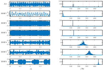
It is assumed that a composite signal contains 4 signals: low-frequency 10Hz signal S₁(t), 130Hz signal S₂(t), 140Hz signal S₃(t), and 450Hz signal S₄(t). The components of the composite signals are either continuous or intermittent in terms of frequency:

$S_{1}(t)=0.1 \cos (2 \pi 10 t)$

$S_{2}(t)=0.5 \cos (2 \pi 130 t)$

$S_{3}(t)=0.5 \cos (2 \pi 140 t)$

$S_{4}(t)=\left\{\begin{array}{lr}0.3 \cos (2 \pi 450 t), & (0 \leq t \leq 0.2 s) \\ 0, & (0.2 \leq t \leq 0.4 s) \\ 0.3 \cos (2 \pi 450 t), & (0.4 \leq t \leq 0.8 s) \\ 0, & (0.8 \leq t \leq 1.1 s) \\ 0.3 \cos (2 \pi 450 t), & (1.1 \leq t \leq 1.45 s) \\ 0, & (1.45 \leq t \leq 1.7 s) \\ 0.3 \cos (2 \pi 450 t), & (1.7 \leq t \leq 2 s)\end{array}\right.$

$S(t)=S_{1}(t)+S_{2}(t)+S_{3}(t)+S_{4}(t)$       (11)

Figure 2 shows the modals after VMD. Among the six modals, BIMF1, BIMF2, BIMF3, and BIMF6 have basically the same features as the original signal, despite having some noises; BIMF4 and BIMF5 correspond to decomposed noise bands, which are not features of the original signal.

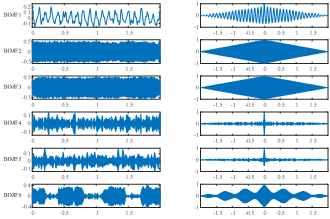
Table 1 lists the ρ_x values of the six modal signals obtained by VMD. Figure 3 shows the autocorrelation functions of the modal signals.

As shown in Table 1 and Figure 3, BIMF4 and BIMF5 had far smaller ρ_x values (close to zero) than other modals. Their SNRs were very poor. Therefore, the two components must be the decomposed noise bands.

During signal reconstruction, the signals of the two noise modals, namely, BIMFs 4 and 5, were removed to obtain the reconstructed signal and its spectrum (Figure 4).

Table 1. Energy ratio of each modal (K=6)

2.png

Figure 2. VMD results of noisy signal

3.png

Figure 3. Autocorrelation functions of modal signals

Figure 4 suggests that the reconstructed signal retained the features of the original signal, and contained much fewer noises, due to the removal of the noise bands of BIMF4 and BIMF5. In other words, the reconstructed signal can retain the features of the original signal and eliminates the noises of that signal through the following steps: calculating the normalized energy ratio of the autocorrelation function for each modal acquired by VMD, setting the corresponding threshold, and selecting modals with high SNR for reconstruction.

4.png

Figure 4. Comparison between reconstructed signal and original signal

To further verify the denoising effect of the improved VMD in different noise backgrounds, the simulated fault signal (11) was added composite noise signals of -5dB, -10dB, and -15dB, respectively, and then decomposed by the improved VMD, EMD, and LMD in turn. Table 2 presents the SNRs of the signals reconstructed by the three methods.

Table 2. Denoising effects of improved VMD, EMD, and LMD in different noise backgrounds

As shown in Table 2, after the simulated fault signal was added composite white noises with different SNRs, the reconstructed signal saw a decline in its SNR, with the enhancement of noise. Under the three different noise backgrounds, the signal reconstructed by the improved VMD had a far higher SNR than EMD and LMD. Under the additive noise of -5dB, the improved VMD led the LMD and EMD by 7.54 and 6.3 in SNR, respectively; under the noise of -10dB, the leads increased to 11.28 and 9.33, respectively; under the noise of -15dB, the leads further grew to 13.3 and 10.97, respectively. In general, the stronger the additive noise, the greater the leads. This means the advantage of the improved VMD in denoising over LMD and EMD increases with the noise intensity.

6205-2RS SKF bearings were selected for fault diagnosis experiments. Local damages were made on the bearings manually with an electric discharge machine. Then, vibration acceleration sensors were installed on the casing at the upper end of the motor output support bearing. After that, the vibration signals were measured at different faults, rotation speeds, and load conditions. The vibration signals were analyzed to identify different fault states.

Improved VMD, EMD, and LMD were separately applied to decompose the data on four different states: normal state, inner ring fault, outer ring fault, and ball fault. A total of 100 data samples were collected for each state. The feature parameters of each dataset were calculated, including variance ν, kurtosis β, and waveform factor S_f. The three characteristic quantities of each dataset were compiled into a 400×3 data matrix, serving as the eigenvector of FCM clustering. The clustering parameters were configured as: the number of cluster heads c=4; fuzzy weight index m=2; convergence precision e=0.001. The clustering results are shown in Figure 5, where each “·” represents a cluster head.

5.png

Figure 5. Clustering effects of different decomposition methods

Figure 5 shows that, after being processed by the FCM algorithm, the 100 datasets were not decomposed, or decomposed by EMD, LMD, and improved VMD, respectively. The clustering results of no decomposition, EMD, and LMD cases had two problems: some samples were far from cluster heads; some fault samples of different classes were mixed together. These problems were the most severe in the no decomposition case, where the clustering effect was the worst, adding to the difficulty of fault sample classification. Meanwhile, the fault samples obtained by improved VMD all gathered around the four cluster heads, with clear boundaries between fault classes. Thus, the improved VMD had much better clustering effect than the other three processing approaches.

To further compare the effects of different decomposition methods, the classification coefficient F, and mean fuzzy entropy H of each method are obtained as shown in Table 3.

Table 3. Fault clustering effects of different decomposition methods

As shown in Table 3, the improved VMD had the largest F value, which was the closest to 1. It was higher than the F values of EMD, LMD, and no decomposition by 0.0879, 0.1223, 0.1365, respectively. The improved VMD also achieved the minimal H value, which was the closest to 0. It was lower than the H values of EMD, LMD, and no decomposition by 0.1847, 0.2455, and 0.2528, respectively. These results demonstrate that the improved VMD has a strong denoising effect, i.e., it can effectively remove the noises from the fault signals of rolling bearings. This effect greatly improves the fault detection ability.