Yingnan Wang* | Yueming Yang | Yan Li
© 2020 IIETA. This article is published by IIETA and is licensed under the CC BY 4.0 license (http://creativecommons.org/licenses/by/4.0/).
OPEN ACCESS
Based on the residual network and long short-term memory (LSTM) network, this paper proposes a human walking gait recognition method, which relies on the vector image of human walking features and the dynamic lower limb model with multiple degrees-of-freedom (DOFs). Firstly, a human pose estimation algorithm was designed based on deep convolutional neural network (DCNN), and used to obtain the vector image of human walking features. Then, the movements of human lower limbs were described by a simplified model, and the dynamic eigenvectors of the simplified model were obtained by Lagrange method, revealing the mapping relationship between eigenvectors in gait fitting. To analyze the difference of human walking gaits more accurately, a feature learning and recognition algorithm was developed based on residual network, and proved accurate and robust through experiments on the data collected from a public gait database.
gait recognition, lower limb motions, residual network, gait difference
Walking distinguishes human from many other animals. It is a complex process of musculoskeletal movement and neural regulation. The research on human walking involves various disciplines, including but not limited to mechanics, kinematics, anatomy, medicine, and psychology. Over the years, human walking analysis has evolved into an important branch of biomechanics called gait analysis. Focusing on human walking movements, gait analysis could summarize the movement law of human body, with the aid of auxiliary instruments, and reveal the kinematics and dynamics of human limbs and joints in the process of walking.
Gait refers to the change of human pose in the process of walking. As a feature of biological behavior, gait can be extracted from a static scene image or a dynamic video sequence. Psychological research shows differences between people in gait. Solely based on gait, many could recognize their friends with an accuracy of 70-80% [1]. Anatomical evidences indicate that the uniqueness of gait comes from the differences in physiological structure, bone length, muscle strength, and walking habits.
In normal environment, healthy people with normal limb functions can walk in a dynamic balance by virtue of their neural regulation system and musculoskeletal movement. Under the effects of internal or external factors, however, an individual might appear unstable in the process of walking. Gait instability is common in our daily life. It might arise from any disturbance of body or environment. To identify gait instability, it is important to identify the biomechanical factors of human lower limbs during stable gait through gait analysis.
This paper mainly recognizes human walking gaits, and analyzes the difference between pedestrians in walking gaits, through intelligent processing of video images. Cutting-edge techniques like residual network, long short-term memory (LSTM) network, deep convolutional neural network (DCNN), and Adam algorithm were combined to realize the research goals. The proposed method was proved valid through experiments on actual gait data, shedding light on gait identification in video sequence.
There are many ways to analyze human gaits, including the traditional footprint method [2], planar fixed-point camera technique [3], and multi-sensor three-dimensional (3D) analysis [4]. Larsen et al. [5] tied light spots to some joints of volunteers, captured the trajectory of the light spots during walking, and recognized the identity and gender of the volunteers based on the captured data. Hak et al. [6] analyzed the walking poses of males and females, and identified gender effectively by the forward swing law of shoulders in the process of walking. These experimental results lay theoretical basis for gait research.
The lower limbs of human have a very complex structure. In the walking process, it is difficult to directly measure the force of each joint and muscle. If these forces could be measured, and used to build the mechanical model of lower limbs, it would be possible to analyze the mechanism of human walking, and develop rehabilitation aids and exoskeleton equipment for lower limbs. Therefore, many researchers have probed into mechanical modeling of the muscles and bones in human lower limbs. For instance, Vairis et al. [7] established a finite-element model of the whole human body, and calculated the stresses of ankle joint and knee joint. With the help of musculoskeletal model, Correa et al. [8] analyzed the stress of lower limb joints, especially the tibia joint, during the walking with different inclinations. Gregg et al. [9] investigated the self-adaptive balancing of human body, which slips in the walking on a straight path, and drew an important conclusion: After slipping, the human body could lighten heel-ground contact and tighten toe-ground contact by reducing the walking speed and step length, and restore stable walking by extending the support phase. Slaughter et al. [10] constructed a forward biomechanical model for the motion system of human lower limbs, which derives the joint torque from the inputted surface electromyography (sEMG) signal, shedding light on the mechanical interaction in human-computer cooperation of rehabilitation training robot.
In gait recognition, image sequence is the basis of most research methods [11]. The image sequence-based methods generally collect gait information over long distance by camera, and identifies the gait through feature extraction and classification. For instance, Chandra et al. [12] successfully recognized gaits with different angles and pedestrian shapes, using the 3D gait data reconstructed by multiple cameras. Kim and Paik [13] combined frieze pattern and dynamic time to match gait sequences with similar angles of view. Lu and Yan [14] classified human contour with hidden Markov model.
Thanks to the development of deep learning, deep neural network (DNN) has been widely applied to gait recognition, for its excellence in feature representation, data learning, and generalization. Carrara et al. [15] designed a human pose estimation model based on convolutional neural network (CNN), relied on the model to obtain the heat map of human joints, and imported the heat map into LSTM network to recognize human poses. Zhu et al. [16] combined three models into a gait recognition method, whose input feature is gait energy map. Kuen et al. [17] developed a gait recognition method coupling multiple progressive stacked auto-encoders: the gait energy map is inputted to multi-layer stacked auto-encoders, and processed progressively to generate gait invariant features.
The generation of vector graph for human walking features is a prerequisite of gait recognition. First, the part affinity fields (PAFs) [18] were extracted by preprocessing gait images. Then, the PAFs of successive frames were combined into the vector graph, which serves as the input of feature extraction and classification network.
To eliminate the influence of background on gait detection, a relatively complete and accurate gait information sequence was obtained from the background images in the video stream. The sequence of the vector graphs in a gait cycle provides sufficient gait information. Hence, this paper proses a gait cycle detection method based on periodic change of aspect ratio of human contour: the PAFs were extracted through gait detection based on pose estimation model, selected for normalization, and organized into a vector graph for human walking features.
Relevant studies have shown that human gait is a highly cyclic behavior. The gait research must learn the change pattern of spatial features. Based on the cyclic information of a gait, a time-scale gait model could be established based on the abundant gait information, which can be trained accurately in a short time.
A gait cycle is defined as the time interval between two consecutive and identical walking poses. In the walking process, the shape of pedestrian contour changes with time, due to the regular movements of arms and legs. The shape changes more sharply in the width direction than in the height direction. That is, the contour variation is most prominent from the side view. Therefore, gait cycles could be extracted based on the aspect ratio, which is maximized when the foot is on the line, and maximized when the foot is fully extended.
In this paper, pedestrian detection is carried out under the you only look once (YOLO) v3 framework [19]. The aspect ratio was acquired from network output [x0, y0, x1, y1] by:
$y_{-} x=y / x$ (1)
where, x=x1-x0; y=y1-y0.
Based on convolutional pose machine, the PAF-based pose estimation [20] can detect the key points of multiple pedestrians in real time. After encoding the global context, the pose estimation algorithm greedily parses the steps from bottom to top. The pedestrians can be recognized precisely and quickly, no matter how many people are in the input image. As a bottom-up method, the algorithm firstly detects the key points in the image, and then connects them according to the position of the human body. In this way, the human pose and gait information can be estimated and extracted successfully, even if the human body is not segmented clearly.
The basic flow of PAF-based pose estimation is as follows: Taking a two-dimensional (2D) w×h RGB image as the input and the positions of key anatomical points for all people in the image as the output, the forward neural network simultaneously predicts the 2D confidence map C of a group of key points, and encodes the 2D vector map V of the correlations between these points. Let C=(C1, C2, …, CM) be a set of M confidence images, each of which corresponds to a key point, with $C_{i} \in \mathbb{R}^{w \times h}, i \in\{1,2, \ldots, M\}$. Let V=(V1, V2, …, VN) be a set of N vector fields, each of which corresponds to a limb, with $V_{j} \in \mathbb{R}^{w \times h \times 2}, j \in\{1,2, \ldots, N\}$. Note that each image position in Vj is encoded as a 2D vector. Next, C and V are analyzed by greedy reasoning, outputting the 2D key points of each person in the image.
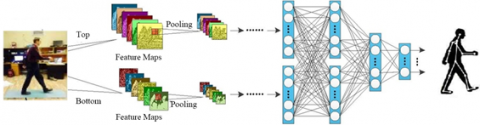
Figure 1. The architecture of two-branch DCNN
Our method was designed based on DCNN. It is not susceptible to background, light, or the number of images. The DCNN could be split into two iterative prediction branches. The top branch predicts confidence maps, while the bottom branch predicts the PAFs of components. As shown in Figure 1, the two-branch DCNN contains t phases, with intermediate supervision between them.
Through the DCNN, a set of feature maps F could be generated from the RGB image, and taken as the input of each branch. From the feature maps, a set of confidence maps C1=β1(F) and a set of PAFs $V^{1}=\vartheta^{1}(F)$ are generated, where β1 and $\vartheta^{1}$ are mapping functions of the DCNN. After each phase, the two branches output their predictions. To improve the prediction accuracy, the predictions and feature maps F are combined as the input of the next phase. This process is implemented iteratively by:
$C^{t}=\beta^{t}\left(F, C^{t-1}, V^{t-1}\right), \forall t \geq 2$ (2)
$V^{t}=\vartheta^{t}\left(F, C^{t-1}, V^{t-1}\right), \forall t \geq 2$ (3)
To guide the iteratively prediction of confidence map and PAFs of key points, each branch has its own loss function in each phase. The loss functions between the true value and the predicted value can be defined as:
$l_{C}^{t}=\sum_{i=1}^{M} \sum_{q} W(q) \cdot\left\|C_{i}^{t}(q)-C_{i}^{*}(q)\right\|_{2}^{2}$ (4)
$l_{V}^{t}=\sum_{j=1}^{N} \sum_{q} W(q) \cdot\left\|V_{j}^{t}(q)-V_{j}^{*}(q)\right\|_{2}^{2}$ (5)
where, $C_{i}^{*}(q)$ is the real confidence map of key points of all pedestrians in the image; W(q)=0 is a binary bit, in which q is not on the joint image; $V_{j}^{*}$ is the real PAFs of all human bodies in the image. The total objective function can be expressed as:
$l=\sum_{t=1}^{T}\left(l_{C}^{t}+l_{V}^{t}\right)$ (6)
As a 2D matrix, the PAF is a strategy to connect the relevant key points correctly, while retaining the position and orientation of limbs. Each pixel in a specific limb could be encoded as a 2D vector from the limb to another limb. The affinity of each limb depends on two key points. Let xi,k and xj,k be the two real body parts i and j of the c-th limb of the k-th person. Then, the affinity vector $L_{c, k}^{*}$ can be defined as:
$L_{c, k}^{*}=\left\{\begin{array}{c}u \text { if } q \text { is on the limb } \\ 0 \quad \text { otherwise }\end{array}\right.$ (7)
The unit vector in limb direction can be expressed as:
$u=\left(x_{j, k}-x_{i, k}\right) /\left\|x_{j, k}-x_{i, k}\right\|_{2}$ (8)
According to the correlation analysis of human anatomical structure, there are 7 degrees-of-freedom (DOFs) in the lower limb on one side of the human body. Hence, the lower limb was simplified as a rigid body model with seven links and seven DOFs. The parameters of this model are shown in Table 1.
Table 1. Parameters of the rigid body model
|
Parameter |
Meaning |
|
θ1, θ2, θ3, θ4, θ5, θ6, θ7 |
Trunk angle, left hip angle, right hip angle, left knee angle, right knee angle, left ankle angle, right ankle angle |
|
mi |
Mass of each link |
|
Ii |
Moment of inertia of each link |
|
li |
Length of each link |
|
di |
Centroid position of each link |
|
kij |
Rigidity of joint muscle |
|
cij |
Rotational damping between adjacent links |
The dynamics of the lower limb system can be generalized as:
$[M]\{\ddot{\theta}\}+[C]\{\dot{\theta}\}+[K]\{\theta\}=[T]$ (9)
This paper aims to model the dynamics of the system. Thus, the damping matrix and external load matrix were set up as [C]=0 and [T]=0, respectively. Then, the dynamic system can be simplified as:
$[M]\{\ddot{\theta}\}+[C]\{\dot{\theta}\}=0$ (10)
The Lagrange equation of the conservative system can be defined as:
$L=T-V$ (11)
$\frac{d}{d t}\left(\frac{\partial L}{\partial \dot{q}_{l}}\right)-\frac{\partial L}{\partial q_{i}}=0$ (12)
where, T and V are the total kinetic energy and total potential energy of the system, respectively; L is Lagrange function about the difference between T and V; qi is the generalized coordinates.
Taking the hip joint as the origin of Cartesian coordinate system, the kinetic energy and potential energy of each limb were expressed in generalized coordinates, and the Lagrange function of the system was established. The Lagrange calculation was performed on the seven generalized coordinates to obtained seven equations.
In the rectangular coordinate system, the coordinates of each node in the simplified model can be expressed as:
$x_{13}=l_{1} \sin \left(\theta_{1}(t)\right)$,
$y_{13}=-l_{1} \cos \left(\theta_{1}(t)\right)$ (13)
$x_{35}=x_{13}-l_{3} \sin \left(\theta_{3}(t)-\theta_{1}(t)\right)$,
$y_{35}=y_{13}-l_{3} \cos \left(\theta_{3}(t)-\theta_{1}(t)\right)$ (14)
$x_{24}=l_{2} \sin \left(\theta_{2}(t)\right)$,
$y_{24}=-l_{2} \cos \left(\theta_{2}(t)\right)$ (15)
$x_{46}=x_{24}-l_{4} \sin \left(\theta_{4}(t)-\theta_{2}(t)\right)$,
$y_{46}=y_{24}-l_{4} \cos \left(\theta_{4}(t)-\theta_{2}(t)\right)$ (16)
The kinetic energy of the left and right lower limbs can be respectively defined as:
$T_{L}=\frac{1}{2} I_{1} \dot{\theta}_{1}^{2}+\frac{1}{2} m_{3}\left(\dot{x}_{13}^{2}+\dot{y}_{13}^{2}\right)+\frac{1}{2} I_{3} \dot{\theta}_{3}^{2}$$+\frac{1}{2} m_{5}\left(\dot{x}_{35}^{2}+\dot{y}_{35}^{2}\right)+\frac{1}{2} I_{5} \dot{\theta}_{5}^{2}$ (17)
$T_{R}=\frac{1}{2} I_{2} \dot{\theta}_{2}^{2}+\frac{1}{2} m_{2}\left(\dot{x}_{24}^{2}+\dot{y}_{24}^{2}\right)+\frac{1}{2} I_{4} \dot{\theta}_{4}^{2}$$+\frac{1}{2} m_{4}\left(\dot{x}_{46}^{2}+\dot{y}_{46}^{2}\right)+\frac{1}{2} I_{6} \dot{\theta}_{6}^{2}$ (18)
The total kinetic energy of the 7-link simplified lower limbs can be expressed as:
$T=\frac{1}{2} I_{0} \dot{\theta}_{0}^{2}+T_{L}+T_{r}$ (19)
The potential energy of the system can be computed by:
$V=\frac{1}{2} k \theta^{2}+\frac{1}{2} k_{1} \theta_{1}^{2}+\frac{1}{2} k_{2} \theta_{2}^{2}+\frac{1}{2} k_{13} \theta_{3}^{2}$$+\frac{1}{2} k_{24} \theta_{4}^{2}+\frac{1}{2} k_{35} \theta_{5}^{2}+\frac{1}{2} k_{46} \theta_{6}^{2}$ (20)
From the above equations of system dynamics, the system dynamics model could be established after computing the equivalent length, equivalent moment of inertia, equivalent limb mass, and rotational rigidity of the simplified 7-link model.
The simplified system (10) can be characterized by the following constitutive equations:
$\left[\begin{array}{ccc}M_{11} & \cdots & M_{17} \\ \vdots & \ddots & \vdots \\ M_{71} & \cdots & M_{77}\end{array}\right]\left[\begin{array}{c}\ddot{\theta} \\ \ddot{\theta}_{1} \\ \ddot{\theta}_{3} \\ \ddot{\theta}_{5} \\ \ddot{\theta}_{2} \\ \ddot{\theta}_{4} \\ \ddot{\theta}_{6}\end{array}\right]+$$\left[\begin{array}{ccccc}k_{0} & & & & & & \\ & k_{1} & & & & & \\ & & k_{13} & & & & \\ & & & k_{35} & & & \\ & & & & k_{2} & & \\ & & & & & k_{24} & \\ & & & & & & k_{46}\end{array}\right]$$\left[\begin{array}{l}\theta_{0} \\ \theta_{1} \\ \theta_{3} \\ \theta_{5} \\ \theta_{2} \\ \theta_{4} \\ \theta_{6}\end{array}\right]=\left[\begin{array}{l}0 \\ 0 \\ 0 \\ 0 \\ 0 \\ 0 \\ 0\end{array}\right]$ (21)
where, $M_{11}=I_{0}$; $M_{22}=I_{1}+m_{5}\left(l_{1}+l_{3}\right)^{2}+m_{3} l_{1}^{2}$; $M_{32}=M_{23}=-m_{5} l_{3}\left(l_{1}+l_{3}\right)$; $M_{33}=I_{3}+m_{5} l_{3}^{2}$; $M_{44}=I_{5}$; $M_{55}=I_{1}+m_{5}\left(l_{1}+l_{3}\right)^{2}+m_{3} l_{1}^{2}$; $M_{65}=M_{56}=-m_{5} l_{3}\left(l_{1}+l_{3}\right)$; $M_{66}=I_{3}+m_{5} l_{3}^{2} ; M_{77}=I_{5}$.
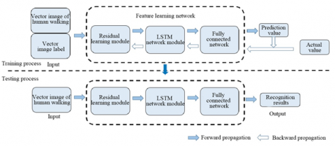
Considering its ultrahigh dimension, the vector image on human walking features must go through dimensionality reduction. Since the PAF image extracted by human pose estimation contain noises, it is necessary to learn the features of the extracted vector image on the spatial scale, so as to facilitate the subsequent feature learning on the time scale. For these purposes, this section proposes a gait feature learning and recognition algorithm based on residual network (Figure 2).
As shown in Figure 2, the vector image on human walking features and the label of the image are adopted as the input of the neural network. In the training process, the residual learning module is adopted to extract spatial features and reduce dimensions. Then, the LSTM network with a special loop is introduced to learn the time scale features. The gait feature representation thus obtained is mapped to the sample label space by the fully connected network, and the features are classified by the softmax layer at the end of the network to obtain the predicted value. Finally, the predicted value is compared with the actual value to derive the cross-entropy loss, and the parameters are optimized by the Adam algorithm with adaptive learning rate. Based on the loss, the backpropagation algorithm is employed to adjust the weight and bias, making the mapping relationship more accurate for feature learning and recognition. During the test, a sequence of vector images on human walking features with the length of a gait cycle is imported to the model for gait identification.
During network training and optimization, the value of each parameter is generally optimized by gradient descent (GD). The backpropagation algorithm makes it efficient to implement GD on every parameter, and minimize the loss function.
Figure 2. Flow chart of feature learning and recognition algorithm based on residual network
Adam algorithm [21] could dynamically adjust the learning rate of each parameter according to the gradient, through first- and second-order moment estimations. Compared with other optimization methods, this algorithm gains high popularity and achieves good performance. In Adam algorithm, the mean sum of squares for gradient exponents st and mean sum of gradient exponents et can be respectively defined as:
$s_{t}=\varepsilon \cdot s_{t-1}+(1-\varepsilon) \cdot g_{t}$ (22)
$e_{t}=\sigma \cdot e_{t-1}+(1-\sigma) \cdot g_{t}^{2}$ (23)
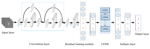
In this paper, a spatiotemporal feature classification model is developed based on network learning and LSTM. The pedestrians are identified through feature learning and prediction of network functions. In the proposed model (Figure 3), the vector image containing spatiotemporal features of human walking is taken as input; the input is processed by a convolution layer with 256 1×1 convolutional kernels; after that, the linear combination of information between channels is changed by Bayesian network (BN) and rectified linear unit (ReLU) nonlinear activation functions [22], which enhances the nonlinear features without loss of resolution, and widens the network channels with the fewest parameters.
In the residual learning module, the number of convolutions is modified, and the position of BN and ReLU is adjusted. Then, dimension reduction is performed through a fully-connected layer. The output of this layer is converted into the input of LSTM network, and the learned feature representation is mapped to the label space of the sample. Finally, the cross-entropy loss is calculated by softmax layer for network training. Through network training and optimization, Adam algorithm is implemented to regularize the loss function to prevent overfitting.
Figure 3. Structure of spatiotemporal gait feature learning and classification network
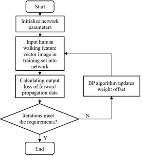
To sum up, the proposed method first calculates the gait cycle, obtains the PAFs, and performs data selection and standardization. Then, the vector image of human walking features is generated. After that, the vector image is adopted as the input in feature learning and recognition based on residual learning module and LSTM network. Through the training, the network capable of extracting spatiotemporal gait features could be obtained. As shown in Figure 4, the specific steps are as follows:
Step 1. From the video sequence of each pedestrian in the dataset, the gait cycle is detected by aspect ratio, and the mean cycle T is obtained. The moving objects are detected and gait information is extracted from the RGB video sequence through human posture estimation, and the PAFs are obtained and standardized. Then, the PAFs in a cycle are superimposed in time sequence, forming a vector of human walking features.
Step 2. The vector image of human walking features is imported to the convolution layer for the exchange of cross-channel information. The feature map is used to extract the spatial features of gait through residual learning module. Then, the outputs of convolution layer and fully-connected layer are sent to the LSTM network to extract the temporal features of gait.
Step 3. Based on the extracted features, the softmax layer at the end of the network is used to classify the features.
Step 4. The cross-entropy loss between the predicted value and the actual value of the softmax layer output is calculated.
Step 5. The network parameters are optimized by backpropagation algorithm according to the cross-entropy loss.
Step 6. Repeat Step 2-5 until the loss error converges.
Figure 4. Workflow of our method
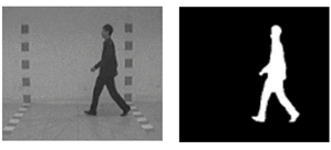
The experimental data were collected from a public gait database. The mean length of gait cycle sequence was taken as the number vector image sequences. Since human pose estimation works poorly on human pose images with large occlusions, the gait sequence from the 50th frame to 50 + Tth frame was taken as the training set from the angle of 0°. Figure 5 presents the recognition effect of our method.
Figure 5. Recognition effect of our method
The recognition effect was measured by the correct recognition rate. The performance of our method was compared with that of two classical recognition algorithms. The comparison in Table 2 shows that our method achieved a mean recognition rate of 96.4%, much higher than the other two algorithms. Hence, our method enjoys strong generalization ability, and surpasses the other methods in eliminating the impact of environmental noise on gait recognition.
Table 2. Correct recognition rates of different algorithms
|
Gait state |
State 1 |
State 2 |
State 3 |
Mean |
|
VGG16 |
100% |
94.6% |
89.2% |
94.6% |
|
Poisson equation + Gabor wavelet |
92.7% |
93.8% |
88.5% |
91.7% |
|
Our method |
100% |
94.5% |
94.7% |
96.4% |
This paper proposes a DCNN-based method for human pose estimation to obtain the vector image on human walking features. Unlike the gait template, the vector image was taken as the gait descriptor that retains all the spatiotemporal features of pedestrians. The abundant gait information in the vector image facilitates the feature extraction and learning, and improves the performance of gait recognition. On this basis, residual learning and LSTM network were combined into a feature learning and recognition network, which has an advantage over traditional machine learning methods in recognition accuracy.
This work is supported by Science and Technology Development Project of Jilin Province (Grant No.: 20190304128YY).
[1] Bashir, K., Xiang, T., Gong, S. (2010). Gait recognition without subject cooperation. Pattern Recognition Letters, 31(13): 2052-2060. https://doi.org/10.1016/j.patrec.2010.05.027
[2] Murukesh, C., Thanushkodi, K., Padmanabhan, P., Feroze, N.M.D. (2014). Secured authentication through integration of gait and footprint for human identification. Journal of Electrical Engineering and Technology, 9(6): 2118-2125. https://doi.org/10.5370/JEET.2014.9.6.2118
[3] Jean, F., Bergevin, R., Albu, A.B. (2005). Body tracking in human walk from monocular video sequences. In The 2nd Canadian Conference on Computer and Robot Vision (CRV'05), Victoria, BC, Canada, pp. 144-151. https://doi.org/10.1109/CRV.2005.24
[4] Naguib, M.B., Madian, Y., Refaat, M., Mohsen, O., El Tabakh, M., Abo-Setta, A. (2012). Characterisation and objective monitoring of balance disorders following head trauma, using videonystagmography. The Journal of Laryngology and Otology, 126(1): 26-33. https://doi.org/10.1017/S002221511100291X
[5] Larsen, P.K., Simonsen, E.B., Lynnerup, N. (2008). Gait analysis in forensic medicine. Journal of Forensic Sciences, 53(5): 1149-1153. https://doi.org/10.1111/j.1556-4029.2008.00807.x
[6] Hak, L., Blokland, I., Houdijk, H. (2020). How do people after stroke adapt step parameters and margins of stability at different walking speeds? Gait & Posture, 81: 136-137. https://doi.org/10.1016/j.gaitpost.2020.07.102
[7] Vairis, A., Petousis, M., Vidakis, N., Kandyla, B., Tsainis, A.M. (2014). Evaluation of a posterior cruciate ligament deficient human knee joint finite element model. QScience Connect, 2014(1): 21. https://doi.org/10.5339/connect.2014.21
[8] Correa, T.A., Baker, R., Graham, H.K., Pandy, M.G. (2011). Accuracy of generic musculoskeletal models in predicting the functional roles of muscles in human gait. Journal of Biomechanics, 44(11): 2096-2105. https://doi.org/10.1016/j.jbiomech.2011.05.023
[9] Gregg, R.D., Tilton, A.K., Candido, S., Bretl, T., Spong, M.W. (2012). Control and planning of 3-D dynamic walking with asymptotically stable gait primitives. IEEE Transactions on Robotics, 28(6): 1415-1423. https://doi.org/10.1109/TRO.2012.2210484
[10] Slaughter, S., Butler, P., Capozzella, H., Nguyen, A., Hutcheson, L. (2012). The comparative gait effects of select walking surfaces using kinetic and EMG analyses. Human Movement, 13(3): 198-203. http://dx.doi.org/10.2478/v10038-012-0022-5
[11] Huang, Q., Cui, L.M. (2019). Design and application of face recognition algorithm based on improved backpropagation neural network. Revue d'Intelligence Artificielle, 33(1): 25-32. https://doi.org/10.18280/ria.330105
[12] Chandra, D., Anggraeni, N.D., Dirgantara, T., Mihradi, S., Mahyuddin, A.I. (2015). Improvement of three-dimensional motion analyzer system for the development of Indonesian gait database. Procedia Manufacturing, 2: 268-274. https://doi.org/10.1016/j.promfg.2015.07.047
[13] Kim, D., Paik, J. (2010). Gait recognition using active shape model and motion prediction. IET Computer Vision, 4(1): 25-36. https://doi.org/10.1049/iet-cvi.2009.0009
[14] Lu, Y., Yan, J. (2020). Automatic lip reading using convolution neural network and bidirectional long short-term memory. International Journal of Pattern Recognition and Artificial Intelligence, 34(1): 2054003. https://doi.org/10.1142/S0218001420540038
[15] Carrara, F., Elias, P., Sedmidubsky, J., Zezula, P. (2019). LSTM-based real-time action detection and prediction in human motion streams. Multimedia Tools and Applications, 78(19): 27309-27331. https://doi.org/10.1007/s11042-019-07827-3
[16] Zhu, X., Yun, L., Cheng, F., Zhang, C. (2020). LFN: Based on the convolutional neural network of gait recognition method. Journal of Physics: Conference Series, 1650(3): 032075. https://doi.org/10.1088/1742-6596/1650/3/032075
[17] Kuen, J., Lim, K.M., Lee, C.P. (2015). Self-taught learning of a deep invariant representation for visual tracking via temporal slowness principle. Pattern recognition, 48(10): 2964-2982. https://doi.org/10.1016/j.patcog.2015.02.012
[18] Wang, H.Y. (2020). Recognition of wrong sports movements based on deep neural network. Revue d'Intelligence Artificielle, 34(5): 663-671. https://doi.org/10.18280/ria.340518
[19] Wu, D., Wu, Q., Yin, X., Jiang, B., Wang, H., He, D., Song, H. (2020). Lameness detection of dairy cows based on the YOLOv3 deep learning algorithm and a relative step size characteristic vector. Biosystems Engineering, 189: 150-163. https://doi.org/10.1016/j.biosystemseng.2019.11.017
[20] Cao, Z., Simon, T., Wei, S.E., Sheikh, Y. (2017). Realtime multi-person 2D pose estimation using part affinity fields. In Proceedings of the IEEE Conference on Computer Vision and Pattern Recognition, pp. 7291-7299. https://arxiv.org/abs/1611.08050
[21] Kumar, V., Laddha, S., Aniket, Dogra, N. (2020). Steganography techniques using convolutional neural networks. Review of Computer Engineering Studies, 7(3): 66-73. https://doi.org/10.18280/rces.070304
[22] Sstla, V., Kolli, V.K.K., Voggu, L.K., Bhavanam, R., Vallabhasoyula, S. (2020). Predictive model for network intrusion detection system using deep learning. Revue d'Intelligence Artificielle, 34(3): 323-330. https://doi.org/10.18280/ria.340310