Lokesh Bhardwaj* | Ritesh Kumar Mishra
© 2020 IIETA. This article is published by IIETA and is licensed under the CC BY 4.0 license (http://creativecommons.org/licenses/by/4.0/).
OPEN ACCESS
The effects of pilot contamination (PC) on the performance of multi-cell multi-user massive multiple input multiple output (MC-MU-m-MIMO) system in uplink has been analyzed in this article. In a multi-cell scenario, the channel estimation (CE) at the desired cell using pilot reuse to avoid significant overhead results in poor CE due to PC. The improvement in degraded performance due to the effect of PC has been shown using low Density Parity Check (LDPC) codes. The comparative analysis of performance in terms of variation in bit error rate (BER) with the signal to noise ratio (SNR) for LDPC coded and uncoded information blocks of users has been shown when the number of cells sharing the same frequency band is varied. Further, the expression for sum-rate has been derived and its variation with the number of base station (BS) antennas has also been shown. The simulated results have shown that the LDPC coded scheme performs better than the uncoded counterpart and the sum-rate capacity increases when the strength of channel coefficients between the BS antennas of the desired cell and the users of remaining cells is less.
massive MIMO, Multi Cell MIMO, low density parity check codes (LDPC), pilot contamination, channel estimation, channel vector
The next generation 5G technology is at the doorsteps to serve the need of an increase in demand of high data rates for a capacious range of applications such as real-time monitoring, vehicle to vehicle communication which have a scope of very low latency. Another important necessity is the usage of spectral efficient systems to provide high speed connectivity so that the crucial resource can be used sagaciously to accommodate a considerable number of subscribers. The probable, reliable, and robust technology capable of serving the above mentioned requisitions is massive multiple input multiple output (m-MIMO) which has considerably large number of BS antennas that are used for accommodating a relatively lesser number of users [1]. It has been proposed that the optimal scheduling of user equipments can increase spectral efficiency (SE) [2]. Thus the technology is termed as multi-user massive MIMO (MU-m-MIMO). Zhang et al. [3] have proposed energy efficient multiple antenna technologies such as cell free massive MIMO, beam space MIMO, and intelligent reflecting surfaces which provide considerably higher gain at a decent cost for enabling the overall scalable connectivity. Murthy and Sankhe [4] have said that spectral efficiency is increased with a confined number of radio frequency chains through a combination of spatial modulation and SM. However, increase in the subscriber base results in limited availability of resources, the same frequency has to be provided in multiple cells resulting in frequency reuse. So, the challenge is to provide connectivity to subscribers present in different cells using the same frequency.
In a typical wireless propagation scenario due to the Rayleigh fading, the signal received is the sum of a large number of multi-path components that differ in phase, time, and amplitude as given in Eq. (1).
$y(t)=s(t) \sum_{i=0}^{Z-1} a_{i} e^{-j 2 \pi f_{c} \tau_{i}}$ (1)
where, Z represents the number of multiple paths, ai and τi are the attenuation and delay of the ith path. s(t) is the transmitted signal. Jerez et al. [5] have proposed a channel model scheme in which dominant multipath components are considered which have a significant impact on the performance of m-MIMO. In m-MIMO, the number of links between a subscriber and a BS is equal to the number of BS antennas. It has been shown that the estimated signal can be obtained from the combined signal version by using efficient MIMO receivers such as matched filter (MF) and zero forcing (ZF) which require the estimation of the channel are given respectively by Eq. (2) [6].
$\tilde{\mathbf{x}}=\mathbf{H}^{H} \mathbf{y}$ and $\tilde{\mathbf{x}}=\left(\mathbf{H}^{H} \mathbf{H}\right)^{-1} \mathbf{H}^{H} \mathbf{y}$ (2)
where, $\tilde{\mathbf{X}}$ is the estimated signal, H and y are the channel matrix and received signal respectively.
It is clear from (2) that CE is utmost crucial in finding $\tilde{\chi}$. If the number of users and pilot symbol vectors for a single cell are K and P respectively, then P≥K so that the pilot matrix becomes orthogonal signifying that the interference between transmitted pilot symbols from K users is zero. However, the orthogonal pilot symbols are optimal when the time slots for pilot training are large enough to support the orthogonality, and if not then the minimum value of error variance shifts from zero to a finite value irrespective of the type of pilot symbols used [7].
In a scenario of L number of multi-cells having a K number of users in each cell as illustrated in Figure 1, if the number of users and pilot vectors required for CE are KL and P respectively, then to maintain orthogonality, the condition P≥KL should be satisfied. This leads to a huge overhead for estimating the channel in MC-MU-m-MIMO as the number of pilot transmission increases by a factor L. If the overhead is avoided by compromising with the orthogonality between pilot symbols, it leads to PC which is due to interference in the pilot from other cells [8]. However, if the ratio of the coherence time of the channel to the number of subscribers in each cell is large, the optimality in the number of pilots also grows resulting in less aggressive pilot reuse [9]. Al-Hubaishi et al. [10] have proposed an effective scheme of assigning the pilot symbols to counter PC when the minimum uplink rate has been maximized and hence inter-cell interference is minimized by considering large-scale characteristics of fading channel. A Hungarian method based optimum pilot allocation scheme has been proposed for maximizing the uplink sum- rate of the system [11].
Figure 1. A typical scenario of MC-MU-m-MIMO system
CE in practical systems is imperfect resulting in CE error having finite variance. This adds to the PC problem and thus the output of the receiver in a multi-cell scenario has some proportion of user information present in L-1 cells along with the desired information resulting in erroneous output at the ZF or MF receiver due to the effect of PC. The signal to interference and noise ratio (SINR) reduces due to additional interference caused by channel vectors of the L-1 cells. For large number of BS antennas, the line of sight (LOS) components is PC free which can be found by the angle of arrivals of signals at users [12]. Akbar et al. [13] have proposed a generalized welch-bound equality (GWBE) base design of pilot sequence for mitigating PC in MC-MU-m-MIMO networks which fulfill the requirements of SINR for all subscribers in the network. Liu et al. [14] have proposed a graph coloring based pilot assignment scheme by utilizing the large-scale coefficients between the access points and user terminals which is capable of reducing the effect of pilot contamination. A method for optimization of coverage, positions, and energy consumption of m-MIMO for low power requirements has been proposed [15]. Al-hubaishi et al. [16] have proposed a partial pilot allocation scheme capable of increasing the uplink rate of users in a multi-cell scenario by exploiting the large- scale characteristics of fading channel so that users having poor channel conditions are saved from harsh interference. Also, with an increase in the number of BS antennas, sum-rate capacity increases as pairwise channel vectors become less correlated [17]. It is very tough to curtail the bit error caused by PC since the separation of desired information from a mess of different signals is challenging. An efficient approach for designing the pilot sequence has been proposed which is capable of achieving capacity and SINR fulfillments for users in presence of PC [18]. It has been proposed by Bhardwaj et al. [19] that the performance degradation in MU-m-MIMO systems with increase in the user base can be overcome by incorporating LDPC codes. Yin et al. [20] have proposed interference free CE performance through covariance aided framework using Bayesian estimator. Some authors have proposed a scheme in which grouping of users can be done in all cells depending on the similarity of the angle of arrivals and by implementing group matching and graph coloring based pilot allocation algorithms, the effect of PC can be minimized [21]. Benzida and Kadochb [22] have suggested the use of raptor codes with minimum mean square estimation (MMSE) to eliminate the use of pilot signals to find the channel state information resulting in reduced BER and power consumption at the user terminal. The problem due to PC can be reduced to some extent through error correction codes (EEC) which are capable of bringing down the BER if the block codes of large length are used. The class of EEC used in this article is LDPC codes which can approach Shannon’s capacity which iterates that reliable communication is possible over an unreliable channel if code rates exceed a specified limit [23]. The iterative procedure helps in obtaining the desired codeword using belief propagation (BP) or sum-product (SP) decoding which uses log-likelihood ratios (LLRs) corresponding to incoming channel information bits. The data bits are encoded by transferring the extrinsic information based on the values of code chart. Another widely used encoding algorithm is dense encoding (DE) technique. Hwang et al. [24] have proposed a lesser complex scheme for improving the m-MIMO performance by jointly detecting and decoding the information that relies on code chart technique. It has been proposed that the error correction coding in MU-m-MIMO systems with phase shift keying outperforms the conventional MIMO technology [25]. Incorporation of orthogonal frequency division multiplexing (OFDM) and LDPC codes with m-MIMO using non-regenerative relays improves the information quality at BS by implementing an MMSE detector with successive interference cancellation (SIC) [26].
In MC-MU-m-MIMO, users are present at different locations in all L cells. The time interval during which the channel impulse response of all the multipath components reaching the BS from a single user is essentially assumed to be constant. Ashikhmin et al. [27] have proposed a large-scale fading precoding concept which can reduce the inter-cell interference significantly by combining the messages aimed at subscribers from various cells that are reusing the training sequence.
A scenario of L multiple cells with an M number of BS antennas and a K number of subscribers in each cell where frequency reuse is implemented to achieve high spectral efficiency to accommodate more users using the same resource is considered for analysis. In Figure 2, the system model has been shown with two cells such that L=2 to present the process flow of signal processing in multiple cells case where cell 1 and cell 2 are considered as desired and interfering cells respectively. The continuous time-varying information signals of K subscribers are converted to unipolar bit streams which are encoded using LDPC codes u11u21…uK1 and u12u23…uK2 represent the information bitstreams of users of cells 1 and 2 respectively. Using LDPC coding, the bitstream corresponding to a user is converted to a codeword. A large block length is used so that the capacity approaching feature of these codes can be exploited as it is crucial in MC-MU-m-MIMO systems since the signals at the output of MIMO receiver is a sum of signals received due to channel coefficients of corresponding users of L cells.
Figure 2. System model of MC-MU-m-MIMO system using LDPC codes showing the information processing at the base station of cell 1 in a 2-cell scenario. Cells 1 and 2 are the desired and interfering cells respectively
Therefore, it is important to employ a scheme that reduces the effect of interference and hence improves the SINR to a considerable extent.
The LDPC Encoder employs DE scheme with coding rate of 1/2 resulting in length n of codeword that is double the bitsream length. Digital carrier modulation schemes used are quadrature amplitude modulation (QAM) and 16-QAM which modulate the encoded vector.
The modulated symbol stream thus created having a length of n/2 or n/4 depending on modulation order of 4 and 16 respectively are transmitted from the subscribers of both cells. The channel coefficients corresponding to the transmitted signals of the first user of the first cell are g111g211…gM11. Additive white gaussian noise (AWGN) gets associated with the composite signal received through the channel coefficients corresponding to the users of both cells at every BS antenna of the first cell.
Each of the M BS antennas receives the symbols of K×2 users of the system. The separation of symbols is done by either ZF or Spatial MF receiver. The separated symbols thus obtained are considered to be the desired symbols of the first cell. However, it is important to realize that these symbols have a share of information transmitted from corresponding users of the second cell due to PC. Demodulation of the symbols obtained at ZF/MF receiver output is done using demodulators of QAM or 16-QAM techniques, whose output is the approximation of original encoded bits. The decoding of the encoded vectors of K users thus obtained is done using the SP/BP algorithm as a part of the LDPC decoding process in which the iterative process increases the chances of reliable decoding. The output of the decoder is the estimated bitstream which is compared with the information bitstream of the user of cell 1 for bit error calculation. In this article, the examination has been done for the proposed model which is extended to L cells for both classical and coded MC-MU-m-MIMO systems with the imperfect channel state information (ICSI) present at the BS.
The main contributions of this study are:
3.1 Single cell MU-m-MIMO
Let’s consider an uplink scenario where a single cell is considered to have a M number of BS antennas and a K number of users. The channel vector M×1 between BS and user k is given as: $\boldsymbol{w}_{k}=\left[\begin{array}{l}w_{1 k} \\ w_{2 k} \\·\\ w_{m k}\\·\\ w_{M k}\end{array}\right]$, here the coefficient of channel between the kth user and mth antenna of the BS is wmk.
wmk ~ CN(0, bk), E{wmk}=0 and $E\left\{\left|w_{m k}\right|^{2}\right\}=b_{k}$, where variance bk models the shadow fading and geometric attenuation.
The considerably large physical distance among users in MU-m-MIMO leads to an existence of time interval during which the channel impulse response between M antennas and a user is fixed.
The M×1 received vector r at the BS is given below in Eq. (3):
$\mathbf{r}=\sqrt{s_{u}}\left[\begin{array}{llll}w_{1} & w_{2} & \ldots & w_{K}\end{array}\right]\left[\begin{array}{l}x_{1} \\ x_{2} \\ \cdot \\ \cdot \\ x_{K}\end{array}\right]+\left[\begin{array}{l}n_{1} \\ n_{2} \\ \cdot \\ \cdot\\ n_{M}\end{array}\right]=\sqrt{s_{u}} \mathbf{W} \mathbf{x}+\mathbf{n}$ (3)
here, W=[w1w2 … wk] is the matrix having channel coefficients between K number of subscribers and M BS antennas. Further, wmk =[W]mk such that entries in W represents the effects of multi-path propagation, log-normal shadowing, and geometric attenuation, and hence it comprises of fast fading due to hmk and large scale fading due to bk. The noise vector n is AWGN noise such that n ~ CN(0,1). A kth user has a symbol xk and the average transmitted power associated with this signal is given by su such that
$\sqrt{s_{u}}\left[\begin{array}{l}x_{1} \\ x_{2} \\ \cdot \\ \cdot \\ x_{K}\end{array}\right]=\sqrt{s_{u}} \mathbf{x}$
where, $\sqrt{s_{u}}$ represents the average strength and $\sqrt{s_{u}} x$ is a column vector simultaneously transmitted by K users. As the BS antennas increases, the mean transmitted power su reduces. For ICSI present at the BS, $s_{u}=1 / \sqrt{M}$, while for accurate channel information, su=1/M [28].
The channel coefficient wmk can thus be represented as $w_{m k}=h_{m k} \sqrt{b_{k}}$ and hence the channel matrix of the form W=HA1/2 is given by Eq. (4) [28].
$\left[\begin{array}{llll}w_{1} & w_{2} & \ldots & w_{K}\end{array}\right]=\left[\begin{array}{llll}\mathbf{h}_{1} & \mathbf{h}_{2} & \ldots & \mathbf{h}_{K}\end{array}\right] \times$
$\left[\begin{array}{ccccc}\sqrt{b_{1}} & 0 & \cdot & \cdot & 0 \\ 0 & \sqrt{b_{2}} & 0 & \cdot & 0 \\ \cdot & 0 & \sqrt{b_{3}} & \cdot & 0 \\ \cdot & 0 & \cdot & \sqrt{b_{k}} & 0 \\ 0 & 0 & . & . & \sqrt{b_{K}}\end{array}\right] \leftarrow \mathbf{A}^{1 / 2}$ (4)
here matrix A is a square matrix that corresponds to geometric attenuation and shadow fading.
3.2 MC-MU-m-MIMO model
Consider a scenario of L multiple cells sharing the same frequency band in an uplink case with M antennas present at the BS and K single antenna users transmitting in every cell. Referring to (3) of section 3.1, the model for a multi-cell scenario is given in Eq. (5).
$\mathbf{r}_{l}=\sqrt{s_{u}} \sum_{j=1}^{L} \mathbf{W}_{l j} \mathbf{x}_{j}+\mathbf{n}_{l}$ (5)
where, rl is the M×1 vector received at the lth BS and Wlj is the channel matrix between lth BS and K users in the jth cell. $\sqrt{S_{u}} \boldsymbol{x}_{j}$ is the K×1 transmitted vector of K users in the jth cell and nl is an AWGN vector having complex normal Gaussian random elements of average power unity at lth BS.
The channel vector at lth BS for ith user present in the jth cell is given by $w_{l j i}=\sqrt{b_{l j i}} h_{l j i}$ where blji represents geometric attenuation and shadow fading between lth BS and the ith user in the jth cell.
The matrix Wlj is therefore given by Eq. (6).
$\mathbf{W}_{l j}=\mathbf{H}_{l j} \sqrt{\mathbf{A}_{l j}}$ (6)
$\mathbf{W}_{l j}=\left[\begin{array}{lllll}\boldsymbol{w}_{l j 1} & \boldsymbol{w}_{l j 2} & \ldots & \boldsymbol{w}_{l j K}\end{array}\right]=\left[\begin{array}{llll}\mathbf{h}_{l j 1} & \mathbf{h}_{l j 2} & \ldots & \mathbf{h}_{l j K}\end{array}\right]\times$
$=\left[\begin{array}{ccccc}\sqrt{b_{l j 1}} & 0 & . & . & 0 \\ 0 & \sqrt{b_{l j 2}} & 0 & . & 0 \\ . & 0 & \sqrt{b_{l j 3}} & . & 0 \\ . & 0 & . & \sqrt{b_{l j k}} & 0 \\ 0 & 0 & . & . & \sqrt{b_{l j K}}\end{array}\right]$
where, Alj is a K×K diagonal matrix such that [Alj]ii= blji.
3.3 Channel estimation in multi cell m-MIMO
Considering a single-cell scenario having K users for which the model for CE at the BS is given in Eq. (7).
$\mathbf{Z}_{M \times K}=\sqrt{K s_{u}}\left[\begin{array}{llll}\boldsymbol{w}_{1} & \boldsymbol{w}_{2} & \ldots & \boldsymbol{w}_{K}\end{array}\right]\left[\begin{array}{llll}\phi_{1} & \phi_{2} & \ldots & \phi_{K}\end{array}\right]+$$\left[\begin{array}{llll}\mathbf{n}_{1} & \mathbf{n}_{2} & \ldots & \mathbf{n}_{K}\end{array}\right]$ (7)
Eq. (7) can be expressed in dimensional form by Eq. (8) [29].
$\mathbf{Z}_{M \times K}=\sqrt{t_{p p}} \mathbf{W}_{M \times K} \mathbf{\phi}_{K \times K}+\mathbf{N}_{M \times K}$ (8)
here ZM×K is the matrix of data aided symbols at the BS. tpp is the power of pilot matrix such that tpp = Ksu. $\phi_{K \times K}$ is matrix of the pilot symbols and $\phi_{k}$ in $\left[\begin{array}{llll}\phi_{1} & \phi_{2} & \ldots & \phi_{K}\end{array}\right]$ is kth vector represented by the K pilot symbols. NM×K represents the noise matrix whose columns represent the noise elements present at M antennas.
The pilot matrix $\phi_{K \times K}$ is chosen in such a way that $\phi \phi^{H}=I$ where I is a K×K identity matrix. The result of this equality leads to orthogonality in the pilot matrix which consequently ends up with minimum or very little interference among the transmitted pilot symbols from different subscribers.
In MC-MU-m-MIMO, the total number of users in L cells is K×L. The CE model for the multi-cell scenario is given in Eq. (9) considering Eq. (8) as the reference equation.
$\mathbf{Z}_{l}=\sqrt{t_{p p}} \sum_{i=1}^{L} \mathbf{W}_{l i} \phi_{i}+\mathbf{N}_{l}$ (9)
here, the number of pilot vectors is PS. Zl and Nl are received and noise matrices having dimensions of M×PS at the lth cell BS. As the number users and BS antennas are assumed to be the same in all cells, the dimensions of matrices Wli and $\phi_{i}$ are M×K and K×PS respectively for all values of i.
Eq. (9) can be put in the form given in Eq. (10).
$\mathbf{Z}_{l}=\sqrt{t_{p p}}\left[\begin{array}{llll}\mathbf{W}_{l 1} & \mathbf{W}_{l 2} & \ldots & \mathbf{W}_{l L}\end{array}\right]\left[\begin{array}{l}\phi_{1} \\ \phi_{1} \\ \vdots \\ \phi_{L}\end{array}\right]+\mathbf{N}_{l}$ (10)
where, [Wl1Wl2 … WlL] is the M×KL channel matrix and $\left[\begin{array}{l}\phi_{1} \\ \phi_{1} \\ \vdots \\ \phi_{L}\end{array}\right]$ is a KL×PS pilot matrix corresponding to L cells. The received matrix can be expressed in the composite form given in Eq. (11).
$\mathbf{Z}_{l}=\sqrt{t_{p p}} \tilde{\mathbf{W}} \tilde{\boldsymbol{\phi}}+\mathbf{N}_{l}$ (11)
In the wireless propagation scenario of L cells, signals from all KL users are being received by the lth BS under consideration. These signals are propagating through different paths which are associated with corresponding channel coefficients. The knowledge of channel coefficients is crucial at the receiver so that signals are separated effectively using the MIMO receiver. The key point is that whether the behavior of the channel is appropriate or abrupt, the estimated coefficients should approach the actual coefficients to get considerable SNR for every received symbol.
3.3.1 Least square estimate
The CE model as given in (11) can be used and Least Square Cost (LSC) function is utilized to get the channel estimate. To obtain the estimate of the channel matrix, the minimum of $\left\|Z_{l}-\tilde{\phi} \widetilde{W}\right\|^{2}$ is evaluated at the receiver for obtaining the output at the MIMO receiver [30].
Estimated channel coefficients after implementation of the LSC function is given in Eq. (12) [31].
$\tilde{\mathbf{W}}=\frac{1}{\sqrt{t_{p p}}} \mathbf{Z}_{l} \tilde{\boldsymbol{\phi}}^{H}\left(\tilde{\phi} \tilde{\phi}^{H}\right)^{-1}$ (12)
It is worth noting from (12) that the orthogonality feature of the pilot matrix is necessary to eliminate the interference among the pilot symbols of KL users. To achieve the orthogonality it is required that $\widetilde{\boldsymbol{\phi}}{\widetilde{\boldsymbol{\phi}}}^{H}=\boldsymbol{I}$. Thus to accomplish the above-mentioned criteria for negligible interference in pilot symbols, the condition in Eq. (13) has to be satisfied.
$P_{s} \geq K L$ (13)
The distinct number of pilot symbols needed for transmission for CE is KL which is same as the total number of users present in a multi-cell scenario. This results in huge overhead in the MC-MU-m-MIMO systems. It is practically difficult to provide such a significant overhead as it may increase the latency caused by the delay in allocation of the orthogonal symbols to the huge user base of L cells. Also for pilot transmission, both allocation of time-frequency resources and coherence time of channel are limited and hence the number of orthogonal pilot symbols is also limited [32].
3.4 Pilot contamination
Avoiding overhead leads to interference in pilot symbols from other cells resulting in PC. The impact of PC on the received signal at the BS of lth cell under consideration can have undesirable implications as the received M×1 vector is the sum of signals from users of L cells and separation process of the information symbols of the desired lth cell users results in the presence of signals from the corresponding users of remaining L-1 cells at the output. This is due to the fact that the channel information present at the lth BS also contains channel fading coefficients of remaining L-1 cells due to PC. Further, as the number of BS antennas increases, the problem of PC may be persistent and the usage of orthogonal symbols might lead to improved performance if the effect of PC is significant [33].
3.4.1 Channel estimation with PC
The number of pilot vectors required for no pilot interference in a multi-cell scenario is KL and one possibility of reducing the overhead is to reuse the pilot matrix in all L cells so that the distinct number of orthogonal pilot symbols required for CE reduces to K as compared to the situation when PC is not considered. Pilot reuse in all cells is given below: $\boldsymbol{\phi}_{j}=\boldsymbol{\phi}_{K \times P_{S}}$ for all values of j.
The CE model with pilot reuse is given in Eq. (14).
$\mathbf{Z}_{l}=\sqrt{t_{p p}} \sum_{j=1}^{L} \mathbf{W}_{l j} \phi+\mathbf{N}_{l}$ (14)
From (14), it is clear that the number of minimal pilot vectors needed is equal to the distinct number of pilot symbols used in the system which is equal to K. So, the overhead is reduced by a factor L that comes at the cost of increased interference since $\boldsymbol{\phi}$ is now reused in all cells. The channel estimated at the lth cell BS using the LSC function is given in Eq. (15).
$\tilde{\mathbf{w}}_{l l}=\frac{1}{\sqrt{t_{p p}}} \mathbf{Z}_{l} \phi^{H}$ (15)
$=\frac{1}{\sqrt{t_{p p}}}\left(\sqrt{t_{p p}} \sum_{j=1}^{L} \mathbf{W}_{l j} \boldsymbol{\phi}+\mathbf{N}_{l}\right) \phi^{H}$ (16)
$=\sum_{j=1}^{L} \mathbf{W}_{l j}+E_{r}$ (17)
where, $E_{r}=\frac{1}{\sqrt{t_{p p}}} \boldsymbol{N}_{l} \phi^{H}$ is the CE error.
The fading coefficients between the K users and the BS of the lth cell include the coefficients from all L cells as mentioned in Eq. (18).
$\tilde{\mathbf{W}}_{l l}=\mathbf{W}_{l l}+\sum_{j=1 \atop j \neq l}^{L} \mathbf{W}_{l j}+E_{r}$ (18)
Here, Wll is the matrix of channel coefficients between K users and M BS antennas of the lth cell. If the ith user in lth cell is the desired user, then the estimated channel vector corresponding to this user is given in Eq. (19).
$\tilde{\boldsymbol{w}}_{l l i}=\boldsymbol{w}_{l l i}+\sum_{j=1 \atop j \neq l}^{L} \boldsymbol{w}_{l j i}+\tilde{\mathbf{n}}_{l}$ (19)
where, the desired channel vector for the ith user of the lth cell is wlli whereas the factor $\sum_{j=1 \atop j \neq l}^{L} \boldsymbol{w}_{l j i}$ representing the effect of PC constitutes corresponding channel vectors of the ith user of L-1 cells. $\tilde{\boldsymbol{n}}_{l}$ is an M×1 noise vector corresponding to Er. In terms of error and the desired channel vector, (19) can be re-written and is given by Eq. (20).
$\tilde{\boldsymbol{w}}_{l l i}=\boldsymbol{w}_{l l i}+\sum_{j=1 \atop j \neq l}^{L} \boldsymbol{w}_{l j i}+\tilde{\mathbf{n}}_{l}=\boldsymbol{w}_{l l i}+\mathbf{e}_{l l i}$ (20)
where, elli is the sum of interfering channel vectors and noise vector $\tilde{\boldsymbol{n}}_{l}$. The desired channel vector wlli of the ith user and $\tilde{\boldsymbol{n}}_{l}$ have variances blli and $\frac{1}{K s_{u}}$ respectively. So, it can be concluded that each element of elli has variance given in Eq. (21).
$\sigma_{e}^{2}=\sum_{j=1 \atop j \neq l}^{L} b_{l j i}+\frac{1}{K s_{u}}$ (21)
The variance in (21) has significance in interference caused at the output of the MIMO receiver. The variance due to multi-cell interference gets added with the variance of CE error to yield high BER when compared to the case of a single cell MU-m-MIMO system. The challenge lies ahead to overcome the effect of PC.
The information is encoded using LDPC codes to ensure a considerably low rate of error at the receiver output. The backend of the encoding process constitutes a parity check matrix having a Bi-Partite graph. A code (8, 4) with rate 1/2 signifies that number of data and parity bits is equal. The corresponding matrix for this code is given in Eq. (22). Data and parity bits are represented by f and n-f respectively.
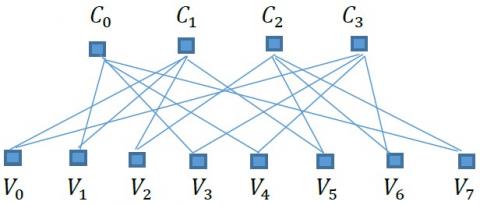
here, F is a parity check matrix which can also be represented by a graphical method known as the Tanner Graph or Bi-Partite graph that has check nodes (C-nodes) and variable (V-nodes). These nodes are connected depending on the intersection of row and column in F. The entry of 1 in F represents the connection of nth variable and mth check node. The Bipartite graph for F is shown in Figure 3 for Eq. (22).
Figure 3. Bipartite graph associated with F~(8, 4)
4.1 Dense LDPC encoding
The f number of data bits are encoded using F which is segregated in two matrices S and T. S is a square matrix which is converted to the non-singular matrix through columns arrangement resulting in a non-zero determinant. The codeword wc is also sub-divided into two subsequences b and d with lengths bL and dL. b and d correspond to parity and data bit sequences having number of bits as n-f and f respectively.
The codeword wc acquired at the output of encoder using F satisfies the condition mentioned in Eq. (23).
$[\mathbf{F}]\left[\mathbf{w}_{c}\right]=0$ (23)
The condition in Eq. (23) processes S and T with A and B:
$[\mathbf{S} \mid \mathbf{T}]\left[\frac{\mathbf{b}}{\mathbf{d}}\right]=0 \Rightarrow[\mathbf{S}][\mathbf{b}]+[\mathbf{T}][\mathbf{d}]=0 \Rightarrow \mathbf{b}=\left[\mathbf{S}^{-1}\right][\mathbf{T}][\mathbf{d}]$
At first, G=[T][d] is calculated following which b=[S]-1[G] is obtained. In general, the parity bits are obtained by translating the matrix [S] to lower or upper triangular matrix for finding b [34]. Using sequence b, a n×1 codeword wc is obtained.
In the MC-MU-m-MIMO system, the 1×f information block corresponding to every user is encoded using LDPC codes of code rate 1/2 to obtain a codeword wc.
4.2 Decoding of Information using BP Decoding
BP or SP uses soft decision by incorporating Log-Likelihood Ratios (LLR). In this algorithm, the messages in terms of LLRs are passed between the V and C nodes. Demodulation of channel information is done to obtain n bits for which Log-Likelihood Ratios (LLRs) are calculated for each V node. LLR is the value in the logarithmic domain which is the probabilistic ratio of a bit having values 0 and 1 if the channel values for respective nodes are known.
Decoding Process
LLRs corresponding to channel bits at V nodes are given in Eq. (24).
$L\left[X_{n} / D_{n}\right]=\ln \left[P_{r}\left(X_{n}=0 / D_{n}\right) / P_{r}\left(X_{n}=1 / D_{n}\right)\right]$ (24)
Dn and L[Xn/Dn] represent the incoming channel bit and the LLR at the nth V node.
The messages in (24) are propagated to the connected C nodes and are given in Eq. (25).
$Z_{n \rightarrow m}\left(X_{n}\right)=L\left(X_{n} / D_{n}\right)$ (25)
where, $Z_{n \rightarrow m}\left(X_{n}\right)$ is the propagated LLR to the mth check from the nth variable node.
The tanh rule is used to update the check nodes by evaluating the LLR which is passed to the connected V node.
Updation is executed by using the messages which are propagated from the V nodes connected to the check node apart from that V node for which the calculation of LLR is being done as shown in Figure 4.
Figure 4. Propagation of LLR to the nth V node from the mth C node
Consider the V nodes associated to V(m):
$P_{m \rightarrow n}\left(R_{m}\right)=L_{m \rightarrow n}\left(R_{m}\right)=\prod_{i=V(m) / n} \operatorname{sign}\left(Z_{i \rightarrow m}\left(X_{i}\right) \times\right.$$2 \tanh ^{-1}\left(\prod_{i=V(m) / n} \tanh \left|Z_{i \rightarrow m}\right| / 2\right)$ (26)
LLR propagated to nth variable from mth check node is represented by $P_{m \rightarrow n}\left(R_{m}\right)$ in Eq. (26) [35] where V(m) represents those V nodes which are linked to mth check and V(m)/n is the number of V nodes connected to mth check node except the nth node to which message has to be propagated. Similarly, updation of all C nodes is done by passing the LLRs to the V nodes.
The LLRs given in Eq. (26) are received by all variable nodes from check nodes.
The LLR for the updated V node is given in Eq. (27).
$Z_{n}\left(X_{n}\right)=L\left(X_{n} / D_{n}\right)+\sum_{m=C(n)} P_{m \rightarrow n}$ (27)
here, the LLR at the nth V node is represented by Zn(Xn) which is the sum of LLRs corresponding to the initial channel bit and the LLRs received from the linked C nodes. C(n) represents the number of check nodes connected to the nth variable node. Eq. (27) concludes the end of the initial iteration [36].
The next iteration means that the messages are passed by the V nodes again back to the C nodes where every V node is updated by using the channel LLRs and the information from all the linked C nodes avoiding only the target C node as depicted in Figure 5.
The updated message to mth check from the nth variable node is given by Eq. (28).
$Z_{n \rightarrow m}\left(X_{n}\right)=L\left[\left(X_{n} / D_{n}\right)\right]+\sum_{j=C(n) / m} P_{j \rightarrow n}\left(R_{j}\right)$ (28)
where, the number of check nodes connected to nth variable node apart from the mth node is represented by C(n)/m. $P_{j \rightarrow n}\left(R_{j}\right)$ is the LLR sent to nth variable from jth check node.
Figure 5. LLR propagation to the mth check from the nth variable node
Codeword check
After the end of every iteration, all the V nodes are updated by acquiring the LLRs as given by Eq. (27).
The quantization of these LLRs is done such that:
If $Z_{n}\left(X_{n}\right)>0 \Rightarrow Z_{n}=0$ else if $Z_{n}\left(X_{n}\right)<0 \Rightarrow Z_{n}=1$
The 1×n processed block corresponding to N variable nodes is given as: $Z=\left[\begin{array}{lllllll}Z_{1} & Z_{2} & Z_{3} & Z_{4} & . & Z_{N}\end{array}\right]$.
The condition F×z’=0 is checked after every iteration and the decoding stops with z as the final output if the condition is satisfied. Further, the algorithm repeats till the convergence is achieved or the set number of iterations are over.
5.1 Analysis of error probability of MC-MU-m-MIMO using LDPC codes
A multi-cell scenario with K users in each cell is considered and a message block Bl for the users present in the lth cell is formed. Bl is a K×f information matrix as given in Eq. (29) with f as the message bits of each user.
$\mathbf{B}_{l}=\left[\begin{array}{ccccc}I_{11} & I_{12} & I_{1 k} & . & I_{1 f} \\ I_{21} & I_{22} & I_{2 k} & . & I_{2 f} \\ . & . & . & . & . \\ I_{K 1} & I_{K 2} & I_{K k} & . & I_{K f}\end{array}\right]$ (29)
here IKk is kth message bit of the user K. DE with coding rate 1/2 is implemented on each row resulting in a codeword with length equal to 2f. The K×n matrix El thus obtained having K codewords is given in Eq. (30).
$\mathbf{E}_{l}=\left[\begin{array}{ccccc}c_{11} & c_{12} & c_{1 k} & \cdot & c_{1 n} \\ c_{21} & c_{22} & c_{2 k} & \cdot & c_{2 n} \\ \cdot & \cdot & \cdot & \cdot & \cdot \\ c_{K 1} & c_{K 2} & c_{K k} & \cdot & c_{K n}\end{array}\right]$ (30)
where, [c11 c12 c1k … c1n] is the codeword obtained for user 1. In a scenario of L cells under consideration, the number of users in all cells is the same and hence the encoded matrices E1, E2, … EL corresponding to L cells have the same dimensions K×n. The modulation of all the codewors of El is done employing QAM and 16-QAM techniques. The K×(n/log2U) modulated matrix Ql thus obtained has modulated symbols and the column vectors are sequentially transmitted by K users. log2U is an integer value (2 or 4) which corresponds to symbol bits and depends on the order of modulation U. The model equation of MC-MU-m-MIMO is thus given in Eq. (31).
$\mathbf{R}_{l}=\sqrt{s_{u}} \sum_{j=1}^{L} W_{l j} \mathbf{Q}_{j}+\mathbf{N}_{l}$ (31)
here, Rl and Nl are M×(n/log2U) received and AWGN noise matrices respectively at the lth cell BS.
Each element of Rl is the summation of symbols obtained from K×L users. Signals separation of the lth cell users is done through ZF receiver giving the output as a K×(n/log2U) block matrix $\hat{\boldsymbol{X}}_{l}$ and is mentioned in Eq. (32), the rows of which represent the estimated symbols of lth cell users in modulated form.
$\hat{\mathbf{X}}_{l}=\left[\begin{array}{ccc}D_{M 1}(1) & D_{M 1}(2) \cdots & D_{M 1}\left(n / \log _{2} U\right) \\ D_{M 2}(1) & D_{M 2}(2) \cdots & D_{M 2}\left(n / \log _{2} U\right) \\ D_{M k}(1) & D_{M k}(2) \cdots & D_{M k}\left(n / \log _{2} U\right) \\ \vdots & \vdots & \vdots \\ D_{M K}(1) & D_{M K}(2) & D_{M K}\left(n / \log _{2} U\right)\end{array}\right]$ (32)
here, DMk(2) is the modulated symbol of second transmission which is expected to be of the kth user of the lth cell at the ZF output. The symbol DMk(2) is given as: DMk(2)= DMk1(2)+ DMk2(2)+…DMkl(2) …+ DMkL(2) where DMk1(2), DMk2(2) and DMkL(2) represent the symbols of kth users of 1, 2, and Lth cells. It clearly represents that DMk(2) also contains the information of the kth user of remaining L-1 cells resulting from PC.
The estimated modulated symbols of $\hat{\boldsymbol{X}}_{l}$ are demodulated to obtain a K×n matrix $\hat{\boldsymbol{B}}_{l}$. The rows of $\hat{\boldsymbol{B}}_{l}$ are the estimated vectors which correspond to codewords of K users of the lth cell. The decoding of every row vector of $\hat{\boldsymbol{B}}_{l}$ is performed through the algorithm as discussed in section 4.2 which gives the output as a K×f block matrix $\widetilde{\boldsymbol{D}}_{l}$. All the row vectors of $\widetilde{\boldsymbol{D}}_{l}$ are the estimated information bitstream of K users of the lth cell under consideration. The comparison of $\widetilde{\boldsymbol{D}}_{l}$ and $\mathbf{B}_{l}$ in terms of bit errors provides the performance analysis of pilot Contaminated MC-MU-m-MIMO system.
Algorithm 1. Analysis of error probability
Initialize SNR and BER
The algorithm executes for L=2,4,6&8
5.2 Sum rate capacity
In this section, the analysis of sum-rate capacity has been done for lth cell users. The expressions of signal to interference and noise ratio (SINR) and capacity are derived for the first user of the lth cell in a scenario of L cells sharing the same frequency band. Thereafter, generalized sum expression for rate will be given for all the K users present in the lth cell.
The modified model equation of the MC-MU-m-MIMO system given in equation 5 can be expressed by Eq. (33).
$\mathbf{r}_{l}=\sqrt{s_{u}}\left(\mathbf{W}_{l 1} \mathbf{x}_{1}+\mathbf{W}_{l 2} \mathbf{x}_{2}+\ldots \mathbf{W}_{l l} \mathbf{x}_{l}+\ldots+\mathbf{W}_{l L} \mathbf{x}_{L}\right)+\mathbf{n}_{l}$ (33)
where, Wll is the channel matrix between M BS antennas and K users of the lth cell. Considering a general case where l=1 in which user 1 is the desired user, so the received vector is given in Eq. (34).
$\mathbf{r}_{1}=\sqrt{s_{u}} \mathbf{W}_{11} \mathbf{x}_{1}+\sqrt{s_{u}}\left(\sum_{j=2}^{L} \mathbf{W}_{1 j} \mathbf{x}_{j}\right)+\mathbf{n}_{1}$ (34)
r1 is M×1 vector received at BS of cell 1.
In terms of channel vector form, the above equation can be rewritten as given in Eq. (35).
$\mathbf{r}_{1}=\sqrt{s_{u}} \mathbf{w}_{111} x_{11}+\sqrt{s_{u}} \sum_{i=2}^{K} \mathbf{w}_{11 i} x_{1 i}+\sqrt{s_{u}} \sum_{j=2}^{L} \sum_{i=1}^{K} \mathbf{w}_{1 j i} x_{j i}+\mathbf{n}_{1}$ (35)
here x11 and x1i are the information symbols of user 1 and ith user of cell 1. xji is the information symbol of the ith user present in the jth cell. w111 is the M×1 vector having fading coefficients between user 1 and M BS antennas of cell 1. w11i is the M×1 channel vector between M BS antennas and ith user of cell 1. w1ji is the M×1 channel vector between M BS antennas of cell 1 and ith user of the jth cell. n1 is the M×1 noise vector at M BS antennas of cell 1.
The received vector r1 is processed at the BS of cell 1 using an MF receiver. The separated signals thus obtained at the output of MF receiver are considered as the symbols of K users of cell 1 which also contain the interfering symbols from remaining L-1 cells. The optimal beamformer for Maximal Ratio Combiner (MRC) for the desired user is $\widetilde{\boldsymbol{W}}_{111}$. Hence the output of spatial MF receiver is thus given by Eq. (36).
Output $_{M F}=\tilde{\mathbf{w}}_{111}^{H} \mathbf{r}_{1}=\tilde{\mathbf{w}}_{111}^{H}\left(\sqrt{s_{u}} \mathbf{w}_{111} x_{11}+\sqrt{s_{u}} \sum_{i=2}^{K} \mathbf{w}_{11 i} x_{1 i}+\right.$$\left.\sqrt{S_{u}} \sum_{j=2}^{L} \sum_{i=1}^{K} \mathbf{w}_{1 j i} x_{j i}+\mathbf{n}_{1}\right)$ (36)
$=\sqrt{s_{u}} \tilde{\mathbf{w}}_{111}^{H} \mathbf{w}_{111} x_{11}+\sqrt{s_{u}} \sum_{i=2}^{K} \tilde{\mathbf{w}}_{111}^{H} \mathbf{w}_{11 i} x_{1 i}+\tilde{\mathbf{w}}_{111}^{H} \mathbf{n}_{1}+$$\sqrt{s_{u}} \sum_{j=2}^{L} \sum_{i=1}^{K} \tilde{\mathbf{w}}_{111}^{H} \mathbf{w}_{1 j i} x_{j i}$ (37)
From (20), the estimated channel vector of user 1 can be written as $\tilde{\boldsymbol{W}}_{111}=\boldsymbol{w}_{111}+\boldsymbol{e}_{111}$, where e111 is the error caused due to the sum of interfering channel vectors of corresponding users of L-1 cells and vector $\tilde{\boldsymbol{n}}_{1}=\left(1 / \sqrt{t_{p p}}\right) \boldsymbol{n}_{1} \phi^{H}$.
The desired signal part in Eq. (37) is $\sqrt{S_{u}} \widetilde{\boldsymbol{W}}_{111}{ }^{H} \boldsymbol{w}_{111} x_{11}$ which can be written as:
$\sqrt{s_{u}} \tilde{\mathbf{w}}_{111}^{H} \mathbf{w}_{111} x_{11}=\sqrt{s_{u}}\left(\mathbf{w}_{111}+\mathbf{e}_{111}\right)^{H} \mathbf{w}_{111} x_{11}$
$=\sqrt{s_{u}}\left\|\mathbf{w}_{111}\right\|^{2} x_{11}+\sqrt{s_{u}} \mathbf{e}_{111}^{H} \mathbf{w}_{111} x_{11}$
The SINR for user 1 present in cell 1is given in Eq. (38).
$\operatorname{SINR}_{11}=\frac{s_{u}\left\|\mathbf{w}_{111}\right\|^{4}}{s_{u} E\left\{\left|\mathbf{e}_{111}^{H} \mathbf{w}_{111}\right|^{2}\right\}+s_{u} \sum_{i=2}^{K} E\left\{\left|\tilde{\mathbf{w}}_{111}^{H} \mathbf{w}_{11 i}\right|^{2}\right\}+}$$S_{u} \sum_{i=1}^{K} \sum_{j=2}^{L} E\left\{\left|\tilde{\mathbf{w}}_{111}^{H} \mathbf{w}_{1 j i}\right|^{2}\right\}+E\left\{\left|\tilde{\mathbf{w}}_{111}^{H} \mathbf{n}_{1}\right|^{2}\right.$ (38)
$\operatorname{SINR}_{11}=\frac{s_{u}\left\|\mathbf{w}_{111}\right\|^{2}}{s_{u} E\left\{\frac{\left|\mathbf{e}_{111}^{H} \mathbf{w}_{111}\right|^{2}}{\left\|\mathbf{w}_{111}\right\|^{2}}\right\}+s_{u} \sum_{i=2}^{K} E\left\{\frac{\left|\tilde{\mathbf{w}}_{111}^{H} \mathbf{w}_{11 i}\right|^{2}}{\left\|\mathbf{w}_{111}\right\|^{2}}\right\}+}$$s_{u} \sum_{i=1}^{K} \sum_{j=2}^{L} E\left\{\frac{\left|\tilde{\mathbf{w}}_{111}^{H} \mathbf{w}_{1 j i}\right|^{2}}{\left\|\mathbf{w}_{111}\right\|^{2}}\right\}+\frac{\left\|\tilde{\mathbf{w}}_{111}\right\|^{2}}{\left\|\mathbf{w}_{111}\right\|^{2}}$ (39)
where, $\widetilde{\boldsymbol{w}}_{111}^{H} \boldsymbol{w}_{11 i}$ is the correlation of the estimated vector of the desired user with the channel vector of the ith user of cell 1. Also
$E\left\{\frac{\left|\mathbf{e}_{111}^{H} \mathbf{w}_{111}\right|^{2}}{\left\|\mathbf{w}_{111}\right\|^{2}}\right\}=\frac{b_{111}\left\|\mathbf{e}_{111}\right\|^{2}}{\left\|\mathbf{w}_{111}\right\|^{2}}=\frac{\left\|\mathbf{e}_{111}\right\|^{2}}{M}$ (40)
where, $\frac{\left\|w_{111}\right\|^{2}}{M}=b_{111}$ is the variance of the channel vector of the desired user as obtained by implementing the law of large numbers.
Further, from (20), $\boldsymbol{e}_{111}=\sum_{j=2}^{L} \boldsymbol{w}_{1 j 1}+\tilde{\boldsymbol{n}}_{1}$ and hence using the Law of large numbers, (40) is modified as follows:
$E\left\{\frac{\left|e_{111}^{H} w_{111}\right|^{2}}{\left\|w_{111}\right\|^{2}}\right\}=\sum_{j=2}^{L} b_{1 j 1}+\frac{1}{K s_{u}}$, here $\sum_{j=2}^{L} b_{1 j 1}$ and $\frac{1}{K s_{u}}$ represent the variances of inter-cell interference due to PC and CE error respectively. Eq. (41) gives the expression for SINR11 by using the above relationship.
$S I N R_{11}=\frac{s_{u}\left\|\mathbf{w}_{111}\right\|^{2}}{s_{u} \sum_{j=2}^{L} b_{1 j 1}+\frac{1}{K}+s_{u} \sum_{i=2}^{K} E\left\{\frac{\left|\tilde{\mathbf{w}}_{111}^{H} \mathbf{w}_{11 i}\right|^{2}}{\left\|\mathbf{w}_{111}\right\|^{2}}\right\}+}$
$S_{u} \sum_{i=1}^{K} \sum_{j=2}^{L} E\left\{\frac{\left|\tilde{\mathbf{w}}_{111}^{H} \mathbf{w}_{1 j i}\right|^{2}}{\left\|\mathbf{w}_{111}\right\|^{2}}\right\}+\frac{\left\|\tilde{\mathbf{w}}_{111}\right\|^{2}}{\left\|\mathbf{w}_{111}\right\|^{2}}$ (41)
$\frac{\left\|\tilde{\mathbf{w}}_{111}\right\|^{2}}{\left\|\mathbf{w}_{111}\right\|^{2}}=\frac{\left\|\tilde{\mathbf{w}}_{111}\right\|^{2} / M}{\left\|\mathbf{w}_{111}\right\|^{2} / M}=\frac{b_{111}+\sum_{j=2}^{L} b_{1 j 1}+\frac{1}{K s_{u}}}{b_{111}}$ (42)
Also, $E\left\{\frac{\left|\tilde{\mathbf{w}}_{111}^{H} \mathbf{w}_{11 i}\right|^{2}}{\left\|\mathbf{w}_{111}\right\|^{2}}\right\}=E\left\{\frac{\left|\tilde{\mathbf{w}}_{111}^{H} \mathbf{w}_{11 i}\right|^{2} / M}{\left\|\mathbf{w}_{111}\right\|^{2} / M}\right\}$
$\Rightarrow E\left\{\frac{\left|\tilde{\mathbf{w}}_{111}^{H} \mathbf{w}_{11 i}\right|^{2} / M}{\left\|\mathbf{w}_{111}\right\|^{2} / M}\right\}=\frac{\left(b_{111}+\sum_{j=2}^{L} b_{1 j 1}+\frac{1}{K s_{u}}\right) b_{11 i}}{b_{111}}$ (43)
Further, $\begin{aligned} E\{&\left\{\begin{array}{l}\left|\tilde{\mathbf{w}}_{111}^{H} \mathbf{w}_{1 j i}\right|^{2} \\ \hline\left\|\mathbf{w}_{111}\right\|^{2}\end{array}\right\}=E\left\{\frac{\left|\tilde{\mathbf{w}}_{111}^{H} \mathbf{w}_{1 j i}\right|^{2} / M}{\left\|\mathbf{w}_{111}\right\|^{2} / M}\right\} \\ &=\frac{\left(b_{111}+\sum_{j=2}^{L} b_{1 j 1}+\frac{1}{K s_{u}}\right) b_{1 j i}}{b_{111}} \end{aligned}$ (44)
Substituting Eqns. (42), (43), and (44) in Eq. (41), the expression for SINR11 in terms of variances of channel vectors is given in Eq. (45).
$SIN{{R}_{11}}=\frac{{{s}_{u}}\parallel {{\mathbf{w}}_{111}}{{\parallel }^{2}}}{{{s}_{u}}\sum\limits_{j=2}^{L}{{{b}_{1j1}}}+\frac{1}{K}+{{s}_{u}}\sum\limits_{i=2}^{K}{\frac{\left( {{b}_{111}}+\sum\limits_{j=2}^{L}{{{b}_{1j1}}}+\frac{1}{K{{s}_{u}}} \right){{b}_{11i}}}{{{b}_{111}}}+}}$
$s_{u} \sum_{i=1}^{K} \sum_{j=2}^{L} \frac{\left(b_{111}+\sum_{j=2}^{L} b_{1 j 1}+\frac{1}{K s_{u}}\right) b_{1 j i}}{b_{111}}+\frac{b_{111}+\sum_{j=2}^{L} b_{1 j 1}+\frac{1}{K s_{u}}}{b_{111}}$ (45)
The expressions given in (43) and (44) are representing intra-cell and inter-cell interference respectively and hence the SINR11 in (45) has been degraded due to the presence of inter-cell interference when compared to a single cell MU-m-MIMO where the factor representing inter-cell interference is nil. The average power of a user su can be scaled as $\frac{E_{u}}{\sqrt{M}}$ where Eu=su using which constant rate can be maintained. So, the expression of asymptotic SINR is given in Eq. (46).
$SIN{{R}_{11}}=\frac{Kb_{111}^{2}E_{u}^{2}}{KE_{u}^{2}\sum\limits_{j=2}^{L}{b_{1j1}^{2}+1}}$ (46)
The rate expression corresponding to SINR11 is given in Eq. (47)
$R_{1}=\log _{2}\left(1+\operatorname{SINR}_{11}\right)$ (47)
The sum-rate expression for K users is given in Eq. (48).
$R=\sum_{i=1}^{K} \log _{2}\left(1+S I N R_{1 i}\right)$ (48)
where, SINR1i represents the SINR of the ith user of cell 1.
In the MC-MU-m-MIMO system, the location of the cell sites is different in a geographical area due to which the power received by the BS of cell 1 from users of L-1 cells is comparatively lesser than that received from users of cell 1. This fact gives an important conclusion on the variance of channel coefficient between M antennas of cell 1 and users of remaining L-1 cells. The shadowing effect leading to large-scale fading increases between two cells which results in a decrease in the power of channel coefficients and hence the variance b1ji reduces due to co-channel cell separation where j and i vary from 2 to L and 1 to K respectively. Hence, the sum-rate capacity can be improved when the large-scale fading increases. Consequently, the separation between two cells where frequency reuse has been implemented has to be sufficiently large so that tolerable SINR is obtained at the BS.
Algorithm 2. Sum-rate of MC-MU-m-MIMO for different receive antennas
The algorithm executes for L=2,4,6&8
The scenario has an uplink transmission of the MC-MU-m-MIMO system having L cells and K=10 is the number of users present in each cell. The number of cells is varied as L=2, 4, 6, and 8 for analysis of performance when PC is considered. The number of receive antennas at every BS is 200. The code rate used is 1/2 for encoding the information block of all users in every cell. LDPC codes improves performance if the block length is large. The information block corresponding to every user has a length equal to 32000 which is capable of reducing the error through an iterative decoding process at the receiver. In general LDPC codes reduces the BER as compared to uncoded case. However, the results have shown how these codes can help reduce the effect of PC in MC-MU-m-MIMO systems. The concatenated scheme is a novel idea that has been discussed and implemented in this work.
In MATLAB simulation, the results are obtained by considering cell 1 as the desired cell and the same pilot matrix is used in every cell which results in significant interference at the BS of cell 1. The number of transmitted symbols for CE is 10.
Figure 6. BER vs SNR for uncoded MC-MU-m-MIMO using QAM for $\sqrt{A_{1 j}} j \in[2, L]=\sqrt{A_{11}}$
Figure 7. BER vs SNR for uncoded MC-MU-m-MIMO using 16-QAM for $\sqrt{A_{1 j}} j \in[2, L]=\sqrt{A_{11}}$
Figure 8. BER vs SNR for LDPC coded MC-MU-m-MIMO using QAM for $\sqrt{A_{1 j}} j \in[2, L]=\sqrt{A_{11}}$
Figure 9. BER vs SNR for LDPC coded MC-MU-m-MIMO using 16-QAM for $\sqrt{A_{1 j}} j \in[2, L]=\sqrt{A_{11}}$
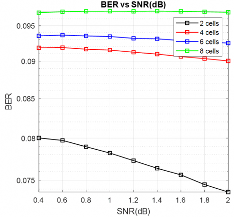
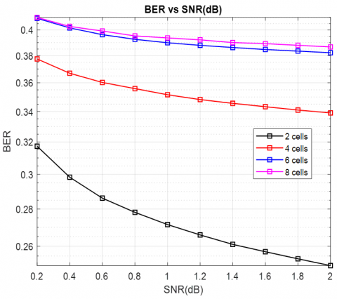
Figures 6 and 7 show the variation in BER when SNR is varied for uncoded signals in uplink scenario case when the digital modulation techniques used are QAM and 16-QAM respectively. Notice that the values 0.37 and 0.41 are the minimum values of BER for L=2 and error increases with the number of cells. The higher value of BER in 16-QAM is due to reduced Euclidean distance between symbols. The overall BER is considerably high due to PC as the number of transmissions of pilot symbol vectors is 10 while the total number of users is L×10.
The performance improvement is seen when LDPC codes are used to encode the information. Figures 8 and 9 show variation in BER with SNR when LDPC codes are used with MC-MU-m-MIMO systems for QAM and 16-QAM modulations techniques respectively.
Initial BER for all values of L is less as compared to the uncoded case while the curves are almost flat for L= 6 and 8. It means that the effect of an increase in SNR has a negligible effect on BER when the number of cells with the same frequency increases due to the huge impact of PC.
The shadow or Log-normal fading increases for the signals received at cell 1 from L-1 cells resulting in reduced strength of channel coefficients. The comparative analysis of performance has been shown when the strength of channel coefficients is same $\sqrt{A_{1 j} j} \in[2, L]=\sqrt{A_{11}}$ and different $\sqrt{A_{1 j} j} \in[2, L] \neq \sqrt{A_{11}}$. Figures 6, 7, 8, and 9 show the performance when the channel strength $\sqrt{A_{1 j}}$ is same for all values of j.
In a more practical scenario where cells are separated spatially due to which the effect of large-scale fading is more and hence the power of the channel coefficients corresponding to cell 1 BS and users of L-1 cells is less.
Figures 10 and 11 show the performance of uncoded scenario when the cells are equidistant and the modulation scheme used is QAM and 16-QAM respectively where channel strength $\sqrt{A_{1 j}}$ is same for $j \in[2, L]$ but is (1/8) of $\sqrt{A_{11}}$. From the Figures 10 and 11, it is evident that the error rate has been reduced when compared with Figures 6 and 7.
LDPC coded case with variable channel coefficients strength has been depicted in Figures 12 and 13 for QAM and 16-QAM respectively.
Figure 10. BER vs SNR for uncoded MC-MU-m-MIMO using QAM for $\sqrt{A_{1 j}} j \in[2, L]=(1 / 8) \sqrt{A_{11}}$
Figure 11. BER vs SNR for uncoded MC-MU-m-MIMO using 16-QAM for $\sqrt{A_{1 j}} j \in[2, L]=(1 / 8) \sqrt{A_{11}}$
Figure 12. BER vs SNR for LDPC coded MC-MU-m-MIMO using QAM for $\sqrt{A_{1 j}} j \in[2, L]=(1 / 8) \sqrt{A_{11}}$
Figure 13. BER vs SNR for LDPC coded MC-MU-m-MIMO using 16-QAM for $\sqrt{A_{1 j}} j \in[2, L]=(1 / 8) \sqrt{A_{11}}$
Figure 14. Uplink sum rate of MC-MU-m-MIMO for $\sqrt{A_{1 j}} j \in[2, L]=(1 / 8) \sqrt{A_{11}}$
Figure 15. Uplink sum rate of MC-MU-m-MIMO for $\sqrt{A_{1 j}} j \in[2, L]=(1 / 8) \sqrt{A_{11}}$
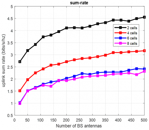
Further, the sum-rate of Pilot contaminated MC-MU-m-MIMO for L=2, 4, 6, and 8 has been shown in Figures 14 and 15 with the variation of rA as [20:30:500] at the BS of cell 1. Figure 14 shows the typical variation in sum-rate when the strength of channel coefficients is same for all values of L. However, Figure 15 shows improvement in sum-rate due to reduced strength of channel $\sqrt{A_{1 j}}$ than $\sqrt{A_{11}}$ where $j \in[2, L]$.
The paper studied two-stage processing of received signal for reducing the error at the BS. The ICSI due to CE error and PC results in huge interference of signals from L-1 cells at the desired BS which separates the signals belonging to K users of the desired cell. The segregated signals also consist of signals of corresponding users present in L-1 cells and therefore the output of the MIMO receiver is decoded using LDPC codes using which significant performance improvement has been shown as error probability has been reduced by (80-85)%. Further, improvement in the performance has been shown when the channel strengths between BS antennas of desired cell and users of remaining cells is less, and hence, the reduction in BER has been observed for both uncoded and LDPC coded system with QAM and 16-QAM respectively. Sum-rates for MC-MU-m-MIMO increase with the number of BS antennas and improve by 60% for the case of reduced strength of channel coefficients. It has been inferred that PC puts a limit on the number of cells which can be given the same frequency as for a higher number of co-channel cells (L= 6, 8) the performance is almost constant even with LPDC codes.
To increase the spectral efficiency in multi-cell MIMO, the number of co-channel cells L increases and PC leads to an increase in inter-cell interference. Further, due to an increase in demand, K also increases which results in performance degradation as the number of antennas at the BS puts a limit on the orthogonality of the channel vectors. A more stringent scheme can therefore be developed which can increase the capacity and spectral efficiency by reusing the frequency while at the same time should reduce the interference so that tolerable SINR can be obtained at the receiver for higher values of L.
[1] Larsson, E.G., Edfors, O., Tufvesson, F., Marzetta, T.L. (2014). Massive MIMO for next generation wireless systems. IEEE Communications Magazine, 52(2): 186-195. https://doi.org/10.1109/MCOM.2014.6736761
[2] Nelluri, M.M.R., Khan, H. (2019). Spectral efficient massive MIMO multi-cell 5G cellular environment using optimal linear processing schemes. International Journal of Recent Technology and Engineering, 7(5S2): 487-491.
[3] Zhang, J., Björnson, E., Matthaiou, M., Ng, D., Yang, H., Love, D.J. (2020). Prospective multiple antenna technologies for beyond 5G. IEEE Journal on Selected Areas in Communications, 38(8): 1637-1660. https://doi.org/10.1109/JSAC.2020.3000826
[4] Murthy, G.R., Sankhe, K. (2016). Spatial modulation-spatial multiplexing in massive MIMO. arXiv:1605.02969v1[cs.IT].
[5] Jerez, J.M.R., Martinez, F.J.L., Martin, J.P.P., Abdi, A. (2019). Stochastic fading channel models with multiple dominant specular components for 5G and beyond. arXiv:1905.03567[cs.IT].
[6] Wang, C., Au, E.K.S., Murch, R.D., Mow, W.H., Cheng, R.S., Lau, V. (2007). On the performance of the MIMO zero-forcing receiver in the presence of channel estimation error. IEEE Transactions on Wireless Communications, 6(3): 805-810. https://doi.org/10.1109/TWC.2007.05384
[7] Wang, H., Zhang, W., Liu, Y., Xu, X., Pan, P. (2015). On design of non-orthogonal pilot signals for a multi-cell massive MIMO system. IEEE Wireless Communications Letters, 4(2): 129-132. https://doi.org/10.1109/LWC.2014.2383382
[8] Boulouird, M., Riadi, A., Hassani, M.M. (2017). Pilot contamination in multi-cell massive-MIMO systems in 5G wireless communications. International Conference on Electrical and Information Technologies (ICEIT), Rabat, pp. 1-4. https://doi.org/10.1109/EITECH.2017.8255299
[9] Sohn, J., Yoon, S.W., Moon, J. (2017). On reusing pilots among interfering cells in massive MIMO. IEEE Transactions on Wireless Communications, 16(12): 8092-8104. https://doi.org/10.1109/TWC.2017.2756927
[10] Al-Hubaishi, A., Noordin, N.K., Sali, A., Subramaniam, S., Mansoor, A.M. (2019). An efficient pilot assignment scheme for addressing pilot contamination in multicell massive MIMO systems. Electronics, 8(4): 372. https://doi.org/10.3390/electronics8040372
[11] Hao, W., Muta, O., Gacanin, H., Furukawa, H. (2019). Uplink pilot allocation for multi-cell massive MIMO systems. IEICE Transactions on Communications, 2: 373-380. https://doi.org/10.1587/transcom.2017EBP3312
[12] Wu, L., Zhang, Z., Dang, J., Wang, J., Liu H., Wu, Y. (2017). Channel estimation for multicell multiuser massive MIMO uplink over Rician fading channels. IEEE Transactions on Vehicular Technology, 66(10): 8872-8882. https://doi.org/10.1109/TVT.2017.2698833
[13] Akbar, N., Yang, N., Sadeghi, P., Kennedy, R.A. (2016). Multi-cell multiuser massive MIMO networks: User capacity analysis and pilot design. IEEE Transactions on Communications, 64(12): 5064-5077. https://doi.org/10.1109/TCOMM.2016.2614674
[14] Liu, H., Zhang, J., Jin, S., Ai, B. (2020). Graph coloring based pilot assignment for cell-free massive MIMO systems. IEEE Transactions on Vehicular Technology, 69(8): 9180-9184. https://doi.org/10.1109/TVT.2020.3000496
[15] Matalatala, M., Deruyck, M., Tanghe, E., Martens, L., Joseph, W. (2018). Optimal low-power design of a multicell multiuser massive MIMO system at 3.7 GHz for 5G wireless networks. Journal on Wireless Communication and Mobile Computing, 2018: 1-17. https://doi.org/10.1155/2018/9796784
[16] Al-hubaishi, A.S., Noordin, N.K., Sali, A., Subramaniam, S., Mansoor A.M., Ghaleb, S.M. (2020). Partial pilot allocation scheme in multi-cell massive MIMO systems for pilot contamination reduction. Energies, 13(12): 3163. https://doi.org/10.3390/en13123163
[17] Wang, D., Ji, C., Gao, X., Sun, S., You, X. (2013). Uplink sum rate analysis of multi-cell multi-user massive MIMO system. IEEE Conference on Communications (ICC), Budapest, pp. 5404-5408. https://doi.org/10.1109/ICC.2013.6655448
[18] Akbar, N., Yan, S., Khattak, A.M., Yang, N. (2020). On the pilot contamination attack in multi-cell multiuser massive MIMO networks. IEEE Transactions on Communications, 68(4): 2264-2276. https://doi.org/10.1109/TCOMM.2020.2967760
[19] Bhardwaj, L., Mishra, R.K., Shankar, R. (2020). Investigation of low-density parity check codes concatenated multi-user massive multiple-input multiple-output systems with imperfect channel state information. The Journal of Defense Modeling and Simulation. https://doi.org/10.1177/1548512920968639
[20] Yin, H., Gesbert, D., Filippou, M.C., Liu, Y. (2013). Decontamination pilots in massive MIMO systems. 2013 IEEE International Conference on Communications (ICC), Budapest, pp. 3170-3175. https://doi.org/10.1109/icc.2013.6655031
[21] Li, P., Gao, Y., Li, Z., Yang, D. (2018). User grouping and pilot allocation for spatially correlated massive MIMO systems. IEEE Access, 6: 47959-47968. https://doi.org/10.1109/ACCESS.2018.2867725
[22] Benzida, D., Kadochb, M. (2018). Raptor code to mitigate pilot contamination in massive MIMO. Procedia Computer Science, 130: 310-317. https://doi.org/10.1016/j.procs.2018.04.044
[23] Richardson, T.J., Urbanke, R.L. (2001). The capacity of low-density parity-check codes under message-passing decoding. IEEE Transactions on Information Theory, 47(2): 599-618. https://doi.org/10.1109/18.910577
[24] Hwang, I., Park, H.J., Lee, J.W. (2019). LDPC coded massive MIMO systems. Entropy, 21(3): 231. https://doi.org/10.3390/e21030231
[25] Roberta, S.C., Carmen, F. (2018). LDPC coding used in massive-MIMO systems. International Conference on Future Access Enablers of Ubiquitous and Intelligent Infrastructures, pp. 52-57. https://doi.org/10.1007/978-3-319-92213-3_8
[26] Berceanu, M., Voicu, C., Halunga, S. (2019). The performance of an uplink massive MIMO OFDM-based multiuser system with LDPC coding when using relays. IEEE 25th International Symposium for Design and Technology in Electronic Packaging, pp. 339-342. https://doi/10.1109/SIITME47687.2019.8990723
[27] Ashikhmin, A., Li, L., Marzetta, T.L. (2018). Interference reduction in multi-cell massive MIMO systems with large-scale fading precoding. IEEE Transactions on Information Theory, 64(9): 6340-6361. https://doi.org/10.1109/TIT.2018.2853733
[28] Kong, C., Zhong, C., Papazafeiropoulos, A.K., Matthaiou, M., Zhang, Z. (2015). Sum-rate and power scaling of massive MIMO systems with channel aging. IEEE Transactions on Communications, 63(12): 4879-4893. https://doi.org/10.1109/TCOMM.2015.2493998
[29] Figueiredo, F., Cardoso, F., Moerman. (2018). Channel estimation for massive MIMO TDD systems assuming pilot contamination and flat fading. EURASIP Journal of Wireless Communications and Network. https://doi.org/10.1186/s13638-018-1021-9
[30] Lioliou, P., Viberg, M. (2008). Least-squares based channel estimation for MIMO relays. International ITG Workshop on Smart Antennas, Vienna, pp. 90-95. https://doi.org/10.1109/WSA.2008.4475542
[31] Neumann, D., Joham M., Utschick, W. (2015). Channel estimation in massive MIMO systems. arXiv: 1503.08691v1[cs.IT], 2015.
[32] Bogale, T.E., Le, L.B. (2014). Pilot optimization and channel estimation for multiuser massive MIMO systems. 48th Annual Conference on Information Sciences and Systems (CISS), Princeton, NJ, pp. 1-6. https://doi.org/10.1109/CISS.2014.6814101
[33] Alkhaled, M., Alsusa, E. (2017). Impact of pilot sequence contamination in massive MIMO systems. IET Communications, 11(13): 2005-2011. https://doi.org/10.1049/iet-com.2017.0062
[34] Richardson, T.J., Urbanke, R.L. (2001). Efficient encoding of low-density parity-check codes. IEEE Transactions on Information Theory, 47(2): 638-656. https://doi.org/10.1109/18.910579
[35] Emran, A.A., Elsabrouty, M. (2014). Simplified variable-scaled min sum LDPC decoder for irregular LDPC codes. 11th IEEE Conference on Consumer Communications and Networking (CCN), Las Vegas, NV, pp. 518-523. https://doi.org/10.1109/CCNC.2014.6940497
[36] Liu, X., Zhang, Y., Cui, R. (2015). Variable-node-based dynamic scheduling strategy for belief-propagation decoding of LDPC codes. IEEE Communications Letters, 19(2): 147-150. https://doi.org/10.1109/LCOMM.2014.2385096