Syed Ahsin Ali Shah* | Nazneen Habib | Malik Sajjad Ahmed Nadeem | Abdulrahman A. Alshdadi | Mohammed Alqarni | Wajid Aziz
© 2020 IIETA. This article is published by IIETA and is licensed under the CC BY 4.0 license (http://creativecommons.org/licenses/by/4.0/).
OPEN ACCESS
The dynamical fluctuations in the Heart Rate Variability (HRV) signals show structures at multiple time scales revealing that complexity of the autonomic nervous system control of the heart is multiscale and hierarchical. Multiscale Entropy (MSE) and its variant Composite MSE (CMSE) were proposed to quantify the complexity at multiple time scales, however, these measures failed to quantify complexity accurately for short duration signals at large temporal scales. To address the downsides of MSE and CMSE, Multiscale Permutation Entropy (MPE) and Improved MPE (IMPE) were proposed. The preliminary results reveal that MPE and IMPE were able to distinguish healthy and pathological subjects, however, further studies are needed to investigate the robustness of these measures. In this study, we investigate the robustness of scale based PE measures in terms of dynamical information, induction of undefined entropy estimates for short duration signals and to classify HRV signals under different physiological and pathological conditions. The results were compared with SE, PE, MSE and CMSE. The MPE and IMPE along with MSE and CMSE provided accurate dynamical information. The results revealed that MPE and IMPE resolved the issue of inducing undefined entropy estimates and are robust in classifying healthy and different pathological subjects.
classification, complexity analysis, heart rate variability, improved multiscale permutation entropy, multiscale permutation entropy
Cardiovascular problems are one of the major causes of mortality across the globe. In 2008, approximately 17.3 million people died due to cardiovascular diseases [1]. According to the World Health Organization (WHO), 30 percent of total global deaths are due to cardiovascular diseases irrespective of geographical boundaries [2]. Therefore, it is very important to identify heart abnormalities at early stages for timely intervention and rehabilitation.
Extraction of physiological and clinical information hidden in biological signals, such as heart rate, respiratory rate, and stride intervals is an important and fascinating field of research [3-7]. Non-invasive assessment of the physiological parameters of a subject enables us to study the physiology and pathophysiology of the investigated system with minimum interference and inconvenience. Electrocardiogram (ECG) is a non-invasive tool that is helpful in continuously monitoring the electrical activity of the heart. Heart Rate Variability (HRV) analysis is performed to study the variations of inter-beat intervals over time which provides important information about the autonomic control of heart [8]. The inter-beat interval (RR-interval) is the time between two consecutive R-peaks of the ECG signal and its reciprocal is called heart rate. HRV reflects the balancing act of sympathetic and parasympathetic branches of the autonomic nervous system to control heart rate. Reduced HRV has been associated with aging and cardiovascular diseases [9].
The underlying mechanism of most of the biological systems is non-linear due to their aperiodic, eccentric, and irregular behavior [3]. The traditional linear times series analysis techniques do not provide appropriate information about the dynamics of physiological systems. With the advent of non-linear dynamical analysis, many researchers have attempted to find the non-linear behavior of the biological systems [3-7]. Extensive scientific efforts have been made for understanding the physiology and pathophysiology of the cardiovascular system. The concept of entropy, first used to measure the disorder of molecules in the field of thermodynamics, is commonly used to understand the physiological systems. A decrease in entropy of the signals received from a system represents the loss of structural and functional complexity, which is a generic feature of aging and pathology [5, 10]. During the last three decades, several entropy-based techniques have been developed by the researchers [11-13].
The complex biological systems exhibit structures at multiple time scales and they function in a dynamic environment. The traditional approaches measure complexity at a single time scale and fail to account for multiple temporal scales inherent in the output signals of these systems [10, 14]. In 2002, Costa et al. proposed Multiscale Entropy (MSE), to represent heart rate dynamics at multiple time scales [10]. Since then, the concept of MSE has become a prevailing method that has been used in diverse fields including biomedical signal processing [10, 15, 16], electro-seismic time series [17], and financial time series [18].
The MSE algorithm relies on the computation of sample entropy [10, 15, 16] of the coarse-grained time series over a sequence of scale factors. The coarse-graining procedure reduces the length of the time series at a scale factor resulting in decreased reliability of entropy estimates or increased probability of undefined entropy values. Wu et al. [19] proposed Composite MSE (CMSE) to address the reliability issue of MSE for short duration time series or at large temporal scales. In the CMSE algorithm, the sample entropies of all coarse-grained time series at a scale factor τ are calculated and the CMSE value is defined as the average of τ sample entropy values [19]. The CMSE provided more reliable entropy estimates but the probability of getting undefined entropy values is increased compared to the MSE. The idea of calculating entropy based on permutation patterns has received considerable attention during the last decade, especially for understanding the dynamics of complex physiological systems. Permutation Entropy (PE) takes the temporal order of the values into account which makes it computationally efficient and robust method to estimate the complexity of time series [13]. Aziz and Arif [20] proposed Multiscale Permutation Entropy (MPE) to improve the classification ability of PE for quantifying the heart rate dynamics. Azami and Escudero [21] proposed Improved Multiscale Permutation Entropy (IMPE) by incorporating the scaling procedure of [19] with PE [16] to increase the stability of MPE.
Awan et al. [14] proposed Multiscale Normalized Corrected Shannon Entropy (MNCSE) to study the dynamics of interbeat interval time series of healthy and diseased subjects. They compared the results of MNCSE with traditional MSE and found that MNCSE is more reliable and stable than MSE. Isler et al. [22] proposed an automatic system using multistage classifiers for diagnosing CHF using short term HRV analysis and obtained an accuracy of 98.8%. For the detection and prediction of 5-minute pre-shock data of CHF, Au-Yeung et al. [23] applied SVM and RF machine learning classifiers and found an accuracy of 81.0% using both classifiers. Sharma et al. [24] employed a time-frequency based method for detecting the presence of Coronary Artery Disease (CAD). They used the extracted features to classify normal ECG beats and CAD using random forest and J48 classifiers and found an accuracy of 99.93%. Li et al. [25] proposed a novel approach for the classification of normal and CHF subjects using a combination of Convolutional Neural Network (CNN) and Distance Distribution Matrix (DDM). They used three CNN models (DenseNet, AlexNet, and SE-Inception-v4), and DDM for the computation of three entropy measures i.e. Fuzzy Global Measure Entropy (FuzzyGMEn), Fuzzy Local Measure Entropy (FuzzyLMEn), and Sample Entropy (SampEn). They found an accuracy of 81.85% using FuzzyGMEn combined with the SE-Inception-v4 model. The studies [22-25] were either conducted for short duration signals or did not investigate the dynamical characteristics of HRV signals. Furthermore these measures did not investigate issue of induction of undefined entropy estimates.
In the present study, at first scale based PE measures, MPE and IMPE, are used to investigate the dynamics of real-world datasets of Normal Sinus Rhythm (NSR) and Congestive Heart Failure (CHF) subjects. Next we investigate the robustness of MPE and IMPE to resolve the issue of induction of undefined entropy estimates for short duration signals and to classify HRV signals under different physiological and pathological conditions. The results of MPE and IMPE are compared with scale based SE measures: MSE and CMSE, for distinguishing healthy and pathological groups as well as to address the problem of undefined entropy estimates. Secondly, scale based PE (PE, MPE, and IMPE) and scale based SE (SE, MSE, CMSE) measures are used to extract featrues from interbeat interval time series data to classify the healthy and diseased subjects. Four different machine learning algorithms (Support Vector Machine (SVM) [26] with the linear and radial kernel (termed as SVM-L and SVM-R respectively), Random Forest (RF) [27], and k-Nearest Neighbour (kNN) [28]) are employed on features extracted using scale based PE and SE measures. The results demonstrated that multiscale based features especially MPE and IMPE are more appropriate in classifying healthy and diseased subjects as well as young and elderly subjects as compared to single scale based features.
In this section, datasets and techniques used in this study are described.
2.1 Datasets
The data used in the study comprises of 72 NSR and 44 CHF subjects, which were taken from publicly available databases from Physionet [29]. There were 35 male and 37 female subjects in the NSR group having 54.6 ± 16.2 (mean ± std) years age. The CHF group comprises of 29 male and 15 female subjects having age 55.5 ± 11.4 years. The NSR data is further divided into young and elderly groups to study the changes in the dynamics of heart rate signals with aging. The young group consists of 26 subjects having ages less than 50 years and elderly subjects composes of 46 subjects having ages greater than 50 years.
The CHF subjects can be categorized into four different groups according to the New York Heart Association (NYHA) functional classification system [30]. The classification of the NYHA system is based on the quality of life of patients and symptoms of everyday activity. For class I, there is no restriction in physical activity whereas for class II there is a very small restriction in physical activity. According to the NHYA system the class I and II are mild classes. In class III subjects, the severity of the disease is moderate and there is a distinct restriction in physical activity. The subjects in class IV are CHF subjects and are unable to move physically and belong to severe disease category. To study the dynamical changes with disease severity, the CHF subjects are divided into two categories. The CHF subjects with lesser disease severity comprises of 12 subjects and belong to NYHA classes I and II while CHF subjects with high disease severity comprises of 32 subjects which belong to NYHA class III and IV.
2.2 Permutation Entropy (PE)
The PE of an arbitrary time series is a complexity measure based on the analysis of permutation patterns of the adjacent values [13]. Embedding theorem indicates that any arbitrary time series $X=\left\{x_{1}, x_{2}, \ldots, x_{m}\right\}$ can be traced on to m dimensional space with vectors $X_{i}=\left\{x_{i}, x_{i+1}, \ldots, x_{i+(m-1) \tau}\right\}$, where m is embedding dimension and τ is the time delay. The patterns of evolution are represented by the components of each vector arranged in ascending order. So the symbolic sequence of the vectors will be the m! i.e., the probable permutations of m divergent symbols. The relative frequency of each permutation pattern π at time delay τ can be determined using the relation
$P_{I}=\frac{\#\left\{t \mid 0 \leq t \leq \tau-m,\left(x_{t+1}, \ldots, x_{t+m}\right) \text { has type } \pi\right\}}{\tau-m+1}$ (1)
The PE of order m≥2 then can be computed using the formula
$\mathrm{PE}=-\sum P_{I} \log P_{I}$ (2)
The PE represents the information contained in a time series data when m consecutive values of that time series are compared.
2.3 Multiscale Permutation Entropy (MPE)
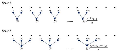
The computation of MPE [20] is based on the construction of the coarse-grained time series using the procedure developed by Costa et al. [15] detailed in Figure 1. The following procedure is used for the computation of MPE.
Step l: For a distinct time series $\left\{t_{i}: i=1,2 \ldots N\right\}$, a set of time series using coarse-grained method is created by averaging the data values within non-coinciding frames of increasing length L. To construct a coarse-grained time sequence following equation is used.
$A_{m}^{(\mathrm{L})}=\frac{1}{L} \sum_{i=(m-1) L+1}^{m L} t_{i}$ (3)
where, L is the scale factor with 1≤m≤N/L. The actual time series length divided by scale factor L gives the coarse-grained time sequence length. Figure 1 demonstrates that the coarse-grained time sequence is distributed into non-coinciding windows of length L, and each window contains the average value of data points.
Step 2: For calculating the MPE, coarse-grained time sequence $\left\{A_{m}: m=1,2 \ldots N\right\}$ is implanted to s dimensional space:
$A_{m}=\{A(m), A(m+\tau), \ldots, A(m+(s-1) \tau)\}$ (4)
Here s is the embedding dimension whereas T represents the time delay. For each m, the existent values $A_{m}=[A(m), A(m+\tau), \ldots \ldots, A(m+(s-1) \tau)]$ of s dimensions can be organized in a cumulative order $\quad[A(m+(m 1-l) \tau \leq A(m+(m 2-1) \tau \ldots \leq A(m+(m s-1) \tau]$. Hence any vector A, is plotted onto $(m 1, m 2, \ldots, m s)$, that is one of the permutations of s diverse signs [1,2,.. .s]. Let, for diverse signs, the probability distribution be PE1, PE2,.PEc, then for the coarse-grained time sequence, the PE is defined as the Shannon Entropy for c diverse signs.
$M P E=-\sum_{u=1}^{c}\left(p E_{u} \ln p E_{u}\right)$ (5)
The length of the time scale is very important as most of the measurements of entropy are reliant on it. The decrease in length of coarse-grained series causes an increase in the variance of measurements of entropy. At greater scales, the approximate error of the MPE algorithm would be high.
2.4 Improved Multiscale Permutation Entropy (IMPE)
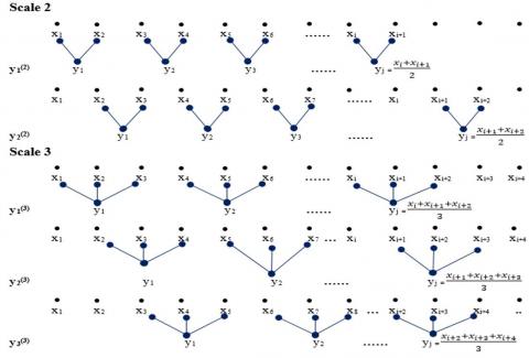
In simple MPE algorithm [20], MPE is calculated using only the first coarse-grained time sequence $A_{1}^{(L)}$, but in IMPE, the PE of all coarse-grained time sequences are computed at every scale factor of L. It is evident from Figure 2 that for scale factors of 2 and 3 there are two and three coarse-grained time sequences, respectively.
For a distinct time sequence $\left\{t_{i}: i=1,2 \ldots N\right\}$, mth time sequence based on the coarse-grained method for some scale factor of L, $y \stackrel{(\mathrm{L})}{m}=y_{m, 1}^{(\mathrm{L})} y_{m, 2}^{(\mathrm{L})} \ldots y_{m, n}^{(\mathrm{L})}$ is defined as
$y_{m}^{(\mathrm{L})}=\frac{1}{L} \sum_{i=(m-1) L+1}^{m L} t_{i} 1 \leq \mathrm{m} \leq \frac{\mathrm{N}}{\mathrm{L}}$ (6)
The IMPE is calculated using the relation
$\operatorname{IMPE}(\mathrm{t}, \mathrm{L}, \mathrm{ord})=1 / \mathrm{L} \sum_{i=1}^{\mathrm{L}} \operatorname{MPE}\left(y_{m}^{(\mathrm{L})}, \text { ord }\right)$ (7)
Figure 1. Schematic illustration of coarse graining procedure [15] for computation of MPE
Figure 2. Schematic illustration of coarse graining procedure [19] for computation of IMPE
2.5 Statistical analysis
Kruskal–Wallis and Mann–Whitney–Wilcoxon (MWW) tests are used to find significant differences among various groups. Kruskal-Wallis test is a non-parametric analog to one-way ANOVA for comparing three or more random independent samples. Kruskal-Wallis test reveals at least one of the groups differs from the remaining groups but does not recognize which pair of groups actually differ. Therefore, for a paired comparison, the Mann-Whitney U test is used to investigate which pair of groups are significantly different. The degree of separation between various groups is assessed using the Area Under Curve (AUC) [31]. The AUC can take any value between 0 and 1, closer the AUC value to 1, better the degree of separation between the groups. The practical lower limit of AUC is 0.5 at which the Receiver Operating Characteristic (ROC) curve will fall to the diagonal and the overall performance of the diagnostic test will rely on pure chance [31].
2.6 Machine learning based classification of HRV signals
Popular machine learning algorithms, SVM (with linear and radial kernels) [26], RF [27], and kNN [28] are used in this study to investigate the efficacy of the features (extracted using scale based measures from HRV signals) in classification of HRV signals. Following is a brief description of each of above mentioned machine learning algorithms.
2.6.1 Support Vector Machine (SVM)
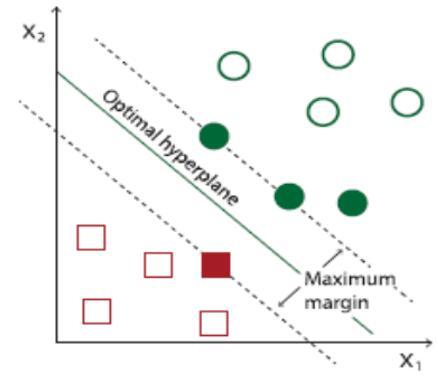
SVM is one of the most widely used algorithm for both linear and nonlinear data classification [26]. SVM basically uses a nonlinear mapping to convert original training data into higher dimensions. It examines the linear hyperplanes for separating data of one class from another one within new dimension. The SVM algorithm selects that hyperplane for which the support vectors (points nearest to the hyperplane on its both sides) have the maximum distance (margin) from the hyperplane. The nonlinear separable data is handled using a kernel function [32], by mapping nonlinear data from input space to the higher dimensional feature space. The most commonly used kernels are linear and radial.
The generic equation for SVM classifier is:
$f(x)=\sum_{i=1}^{l}\left(\alpha_{i}-\alpha_{i}^{*}\right) k\left(x_{i}, x\right)+b$ (8)
k(xi, x) indicates the kernel function. The mathematical representation of linear and radial kernel functions used in this study are as follows.
Linear: $k\left(x_{1}, x_{2}\right)=x_{1}^{T} x_{2}$ (9)
Radial: $k\left(x_{1}, x_{2}\right)=e^{-\gamma\left\|x_{1}-x_{2}\right\|^{2}}$ (10)
The geometric definition of SVM is represented in Figure 3. Figure is retrieved from Toledo-Pérez’s study [33].
2.6.2 Random Forest (RF)
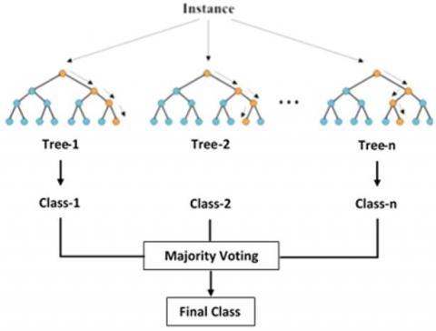
RF is a flexible and efficient algorithm which constructs various decision tree models and merges them together for reliable and accurate prediction [27]. The accuracy of RF models depends on strength of individual trees in the forest as well as the correlation between them. The generalization error is reduced when the individual trees are more accurate for prediction. In order to forecast a new sample from an input vector, the new sample is positioned at the end of each tree in the forest. Each tree gives a predicted value and the final predicted value is the one which is selected by the forest based on maximum votes from all trees. RF classifier with n decision trees is illustrated in Figure 4. Figure is retrieved from Gajja’s study [34].
2.6.3 k-Nearest neighbor
kNN algorithm [28] is based on distance function (e.g. Euclidean distance) and is used to classify data with respect to their k nearest neighbors [35]. It is based on learning by similarity i.e. by doing a comparison of test tuple with training tuples. A descriptive example of kNN classifier which supports three classes A, B, and C with k=7 is illustrated in Figure 5. The point Xt will be classified to class B. Figure is retrieved from Atallah’s study [36].
Figure 3. Generic definition of SVM
Figure 4. RF classifier example
Figure 5. kNN classifier example
2.6.4 Leave One Out Cross Validation (LOOCV)
The LOOCV is a method used to investigate the genralized classification ability of models for the problems where the number of samples for each class are extremely small. In this study, we have 72 NSR and 44 CHF subjects in the available dataset which is considered as extremely small dataset. LOOCV is used here for the formulation of training/testing data and parameter optimization. In LOOCV one of the samples is used to test the performance of the predictive model while the rest of the samples are used to construct the predictive model. This procedure is repeated for all the samples in the available dataset and every time only a single sample is used for performance evaluation. In this way, the performance of the predictive models is measured for all the samples in the available dataset.
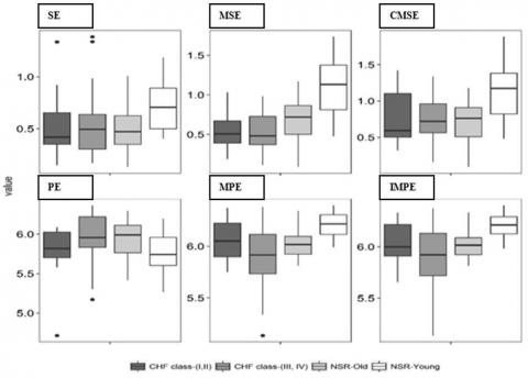
In Figure 6, the distributional characteristics of NSR-young, NSR-old, CHF class-(I, II), and CHF class-(III, IV) subjects using a scale based SE and PE at optimal pattern length/order are presented in the form of a boxplot. The middle line inside each box is the median value, while the edges of the box represent 25th and 75th percentile and points outsides the whiskers represented by a dot are outliers. It is evident from the Figure 6 that the degree of overlap is higher between various groups for SE and PE (entropies computed at temporal scale 1) as compared to scale based version of SE and PE. The scale based SE and PE manifest obvious differences between healthy subjects and physiological disturbances caused by aging or disease.
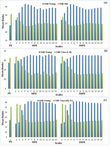
In Figure 7 (a, b, c), results of PE, MPE, and IMPE in terms of mean ranks and in Table 1, their corresponding p-values at temporal scales 1 to 15 are presented. Higher mean rank corresponds to higher entropy estimates representing physiologically complex signals. The PE assigned higher mean ranks to NSR-old, CHF class-(I, II) and CHF class-(III, IV) subjects than NSR-young subjects, representing incorrect information about the dynamics of these systems. Whereas, scale based PE measures assigned higher entropy values to NSR-young subjects at higher temporal scales indicating healthy dynamics are more complex, refuting the original PE algorithm. MPE and IMPE significantly distinguishes healthy from pathological and elderly subjects at wide range of temporal scales. The findings indicate that both time scale and specific entropy values need to be taken into account for better characterization of physiological processes.
In Figure 8 (a, b, c), results of SE, MSE, and CMSE in terms of mean rank and in Table 2, their corresponding p-values for distinguishing healthy from pathological subjects are presented. Higher mean rank corresponds to higher entropy values manifesting more complex dynamics of the underlying system. It is evident from the Figure that the mean ranks of NSR-young subjects are higher than NSR-old, CHF class-(I, II) and CHF class-(III, IV) subjects at all the temporal scales including scale 1 i.e. simple SE. The MSE and CMSE are able to distinguish NSR-young from other groups more significantly at a wide range of temporal scales compared to SE.
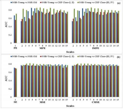
In Figure 9 (a, b), the values of AUC for assessing the degree of separation of scale based PE and SE at different temporal scales for distinguishing healthy subjects from pathological and elderly subjects are presented. The AUC is a generally distinguished index showing the degree of separation among the groups. The AUC values show perfect separation between two groups at a maximum value that is ‘1’ and AUC value ‘0.5’ correspond to the separation between groups by pure chance. It is evident from the Figure that AUC values for both scale based PE and SE are considerably high as compared to PE and SE. The maximum separation between NSR-young and NSR-old subjects for both MPE and IMPE is obtained at scale 5 (AUC value = 0.85 & 0.84 respectively), whereas the maximum separation among NSR-young and CHF class-(I, II) subjects is achieved at scale 13 and 7 (AUC value = 0.78 & 0.76 respectively). The optimal separation among NSR-young and CHF class-(III, IV) subjects is obtained at scale 7 (AUC value = 0.86). In the case of MSE and CMSE, the optimal separation between NSR-young and NSR-old subjects is achieved at scale 13 (AUC value = 0.79), whereas the optimal separation between NSR-young and CHF class-(I, II) subjects is obtained at scale 3 (AUC value = 0.78 & 0.79). The optimum separation among NSR-young and CHF class-(III, IV) subjects for both MSE and CMSE is achieved at scale 4 (AUC value = 0.82 & 0.81). The results indicate that the degree of separation between NSR and CHF subjects increased with disease severity. It is also clear from Figure 9 (a, b) that scale based PE provides better separation compared to scale based SE at multiple time scales.
In Table 3, the robustness of scale based PE measures for assessing the dynamics of time series data of different lengths is illustrated. The mean ± std values of MPE, IMPE, MSE, and CMSE at temporal scales 1 to 15 at specific length are compared. The results indicate that the standard deviation of MPE and IMPE values at different lengths is lower than the standard deviation of MSE and CMSE. Thus, MPE and IMPE lead to more consistent entropy estimates compared to MSE and IMSE. As shown in the Table 3, MSE induced the undefined entropy values at large temporal scales for time series data of short lengths, and CMSE even induced much more undefined entropy values compared to original MSE, whereas, MPE and IMPE eliminated the probability of inducing undefined entropy estimates. The results depict that scale based PE measures are superior than scale based SE measures regarding the validity of entropy estimates for short duration time series at large scale factors.
Table 1. p-values for paired comparison of NSR-Young vs NSR-Old, NSR-Young vs CHF Class-(I, II) and NSR-Young vs CHF Class-(III, IV) groups
|
Scale |
NSR-Young vs NSR-Old |
NSR-Young vs CHF Class-(I,II) |
NSR-Young vs CHF Class-(III,IV) |
|||
|
|
PE |
|||||
|
1 |
8.06×10-03 |
5.10×10-01 |
3.13×10-03 |
|||
|
|
MPE |
IMPE |
MPE |
IMPE |
MPE |
IMPE |
|
2 |
5.11×10-01 |
4.89×10-01 |
3.62×10-01 |
3.46×10-01 |
9.66×10-06 |
9.66×10-06 |
|
3 |
5.75×10-02 |
7.10×10-02 |
8.51×10-01 |
8.51×10-01 |
8.69×10-05 |
9.89×10-05 |
|
4 |
7.79×10-05 |
5.24×10-05 |
3.79×10-01 |
2.86×10-01 |
3.02×10-01 |
2.95×10-01 |
|
5 |
4.63×10-07 |
7.08×10-07 |
7.86×10-02 |
1.16×10-01 |
4.10×10-04 |
5.19×10-04 |
|
6 |
1.01×10-06 |
1.14×10-06 |
2.38×10-02 |
1.70×10-02 |
4.63×10-06 |
6.70×10-06 |
|
7 |
5.10×10-06 |
1.29×10-05 |
6.29×10-03 |
1.00×10-02 |
1.85×10-06 |
2.16×10-06 |
|
8 |
6.08×10-05 |
8.59×10-05 |
1.43×10-02 |
7.60×10-03 |
7.21×10-06 |
4.63×10-06 |
|
9 |
9.07×10-04 |
3.65×10-04 |
2.01×10-02 |
1.10×10-02 |
1.38×10-05 |
6.70×10-06 |
|
10 |
3.49×10-04 |
1.75×10-03 |
9.15×10-03 |
1.10×10-02 |
6.23×10-06 |
2.26×10-05 |
|
11 |
1.89×10-03 |
1.55×10-03 |
4.12×10-02 |
1.31×10-02 |
1.29×10-05 |
4.49×10-05 |
|
12 |
9.86×10-04 |
9.46×10-04 |
1.20×10-02 |
1.56×10-02 |
5.49×10-05 |
5.49×10-05 |
|
13 |
3.05×10-04 |
4.17×10-04 |
3.86×10-03 |
1.20×10-02 |
3.20×10-05 |
7.15×10-05 |
|
14 |
1.84×10-04 |
3.05×10-04 |
1.10×10-02 |
1.20×10-02 |
6.69×10-05 |
1.06×10-04 |
|
15 |
3.49×10-04 |
1.68×10-04 |
2.58×10-02 |
1.70×10-02 |
3.86×10-04 |
1.75×10-04 |
Table 2. p-values for paired comparison of NSR-Young vs NSR-Old, NSR-Young vs CHF Class-(I,II) and NSR-Young vs CHF Class-(III,IV) groups
|
Scale |
NSR-Young vs NSR-Old |
NSR-Young vs CHF Class-(I, II) |
NSR-Young vs CHF Class-(III,IV) |
|||
|
|
SE |
|||||
|
1 |
5.20×10-04 |
3.27×10-02 |
4.43×10-03 |
|||
|
|
MSE |
CMSE |
MSE |
CMSE |
MSE |
CMSE |
|
2 |
2.57×10-05 |
3.50×10-05 |
7.60×10-03 |
7.60×10-03 |
9.89×10-05 |
8.69×10-05 |
|
3 |
1.69×10-05 |
1.98×10-05 |
3.16×10-03 |
2.85×10-03 |
3.20×10-05 |
2.99×10-05 |
|
4 |
1.98×10-05 |
2.85×10-05 |
6.92×10-03 |
6.29×10-03 |
1.20×10-05 |
1.59×10-05 |
|
5 |
4.07×10-05 |
4.07×10-05 |
4.27×10-03 |
4.27×10-03 |
2.60×10-05 |
2.26×10-05 |
|
6 |
3.68×10-05 |
3.16×10-05 |
5.19×10-03 |
5.19×10-03 |
2.43×10-05 |
2.43×10-05 |
|
7 |
2.31×10-05 |
2.31×10-05 |
1.10×10-02 |
5.72×10-03 |
5.49×10-05 |
3.92×10-05 |
|
8 |
2.85×10-05 |
1.88×10-05 |
8.34×10-03 |
5.19×10-03 |
4.20×10-05 |
4.20×10-05 |
|
9 |
1.44×10-05 |
2.20×10-05 |
1.10×10-02 |
9.15×10-03 |
5.13×10-05 |
5.49×10-05 |
|
10 |
6.37×10-06 |
1.44×10-05 |
1.31×10-02 |
1.00×10-02 |
6.26×10-05 |
6.69×10-05 |
|
11 |
3.16×10-05 |
1.16×10-05 |
1.10×10-02 |
1.00×10-02 |
1.75×10-04 |
1.28×10-04 |
|
12 |
8.39×10-06 |
9.36×10-06 |
1.43×10-02 |
1.00×10-02 |
1.75×10-04 |
9.89×10-05 |
|
13 |
7.94×10-06 |
8.86×10-06 |
1.31×10-02 |
1.10×10-02 |
1.75×10-04 |
1.36×10-04 |
|
14 |
8.39×10-06 |
1.16×10-05 |
3.82×10-02 |
1.31×10-02 |
2.86×10-04 |
1.55×10-04 |
|
15 |
1.36×10-05 |
1.23×10-05 |
3.02×10-02 |
1.31×10-02 |
1.86×10-04 |
3.04×10-04 |
Table 3. Mean ± Std of various entropy estimates for NSR young subjects using different data lengths
|
Data Length |
||||||||
|
Scale |
2000 |
4000 |
6000 |
8000 |
||||
|
MSE |
MPE |
MSE |
MPE |
MSE |
MPE |
MSE |
MPE |
|
|
1 |
0.44±0.2 |
0.95±0.04 |
0.51±0.21 |
0.95±0.04 |
0.56±0.23 |
0.93±0.04 |
0.59±0.21 |
0.93±0.04 |
|
2 |
0.28±0.18 |
0.94±0.05 |
0.55±0.21 |
0.93±0.04 |
0.59±0.24 |
0.93±0.03 |
0.63±0.22 |
0.93±0.04 |
|
3 |
0.41±0.21 |
0.94±0.03 |
0.61±0.25 |
0.93±0.03 |
0.56±0.25 |
0.95±0.03 |
0.66±0.22 |
0.94±0.04 |
|
4 |
0.39±0.23 |
0.96±0.02 |
0.54±0.24 |
0.95±0.03 |
0.61±0.26 |
0.97±0.02 |
0.65±0.21 |
0.95±0.03 |
|
5 |
NaN |
0.97±0.02 |
0.49±0.22 |
0.97±0.02 |
0.54±0.24 |
0.96±0.02 |
0.68±0.22 |
0.97±0.02 |
|
6 |
NaN |
0.97±0.01 |
0.43±0.23 |
0.96±0.02 |
0.53±0.25 |
0.97±0.02 |
0.67±0.22 |
0.97±0.02 |
|
7 |
NaN |
0.97±0.01 |
0.49±0.22 |
0.97±0.01 |
0.57±0.24 |
0.97±0.02 |
0.68±0.22 |
0.98±0.01 |
|
8 |
NaN |
0.98±0.01 |
0.45±0.22 |
0.97±0.02 |
0.44±0.2 |
0.97±0.02 |
0.67±0.21 |
0.97±0.02 |
|
9 |
NaN |
0.97±0.02 |
NaN |
0.97±0.02 |
0.53±0.23 |
0.97±0.02 |
0.64±0.2 |
0.97±0.02 |
|
10 |
NaN |
0.97±0.02 |
NaN |
0.98±0.01 |
0.43±0.2 |
0.97±0.02 |
0.67±0.21 |
0.98±0.02 |
|
11 |
NaN |
0.97±0.02 |
NaN |
0.97±0.02 |
NaN |
0.97±0.02 |
0.62±0.19 |
0.98±0.01 |
|
12 |
NaN |
0.98±0.02 |
NaN |
0.98±0.02 |
NaN |
0.97±0.02 |
0.65±0.2 |
0.98±0.01 |
|
13 |
NaN |
0.97±0.02 |
NaN |
0.97±0.02 |
NaN |
0.98±0.02 |
0.62±0.19 |
0.97±0.02 |
|
14 |
NaN |
0.97±0.02 |
NaN |
0.97±0.02 |
NaN |
0.97±0.02 |
0.66±0.2 |
0.98±0.01 |
|
15 |
NaN |
0.97±0.02 |
NaN |
0.97±0.02 |
NaN |
0.97±0.02 |
0.65±0.2 |
0.98±0.02 |
|
Scale |
2000 |
4000 |
6000 |
8000 |
||||
|
CMSE |
IMPE |
CMSE |
IMPE |
CMSE |
IMPE |
CMSE |
IMPE |
|
|
1 |
0.44±0.2 |
0.95±0.04 |
0.51±0.21 |
0.95±0.04 |
0.56±0.23 |
0.94±0.04 |
0.59±0.21 |
0.93±0.04 |
|
2 |
0.33±0.19 |
0.94±0.04 |
0.56±0.22 |
0.93±0.04 |
0.59±0.24 |
0.93±0.04 |
0.58±0.23 |
0.93±0.04 |
|
3 |
NaN |
0.94±0.03 |
0.54±0.23 |
0.93±0.03 |
0.57±0.25 |
0.93±0.03 |
0.59±0.24 |
0.94±0.04 |
|
4 |
NaN |
0.96±0.02 |
0.59±0.27 |
0.95±0.03 |
0.58±0.25 |
0.95±0.03 |
0.6±0.25 |
0.96±0.03 |
|
5 |
NaN |
0.97±0.02 |
0.53±0.23 |
0.97±0.02 |
0.56±0.25 |
0.97±0.02 |
0.57±0.24 |
0.97±0.02 |
|
6 |
NaN |
0.98±0.01 |
0.55±0.24 |
0.97±0.02 |
0.59±0.25 |
0.97±0.02 |
0.59±0.25 |
0.97±0.02 |
|
7 |
NaN |
0.98±0.01 |
NaN |
0.97±0.02 |
NaN |
0.97±0.02 |
0.54±0.23 |
0.98±0.01 |
|
8 |
NaN |
0.98±0.01 |
NaN |
0.97±0.02 |
0.54±0.22 |
0.97±0.02 |
0.59±0.24 |
0.97±0.02 |
|
9 |
NaN |
0.98±0.01 |
NaN |
0.97±0.02 |
0.57±0.22 |
0.97±0.02 |
0.6±0.23 |
0.97±0.01 |
|
10 |
NaN |
0.98±0.02 |
NaN |
0.97±0.02 |
NaN |
0.97±0.02 |
NaN |
0.97±0.01 |
|
11 |
NaN |
0.98±0.02 |
NaN |
0.97±0.01 |
NaN |
0.97±0.02 |
NaN |
0.97±0.01 |
|
12 |
NaN |
0.98±0.02 |
NaN |
0.97±0.02 |
NaN |
0.97±0.02 |
NaN |
0.97±0.01 |
|
13 |
NaN |
0.98±0.02 |
NaN |
0.97±0.02 |
NaN |
0.98±0.02 |
NaN |
0.97±0.01 |
|
14 |
NaN |
0.98±0.02 |
NaN |
0.98±0.02 |
NaN |
0.98±0.02 |
NaN |
0.98±0.01 |
|
15 |
NaN |
0.98±0.02 |
NaN |
0.98±0.02 |
NaN |
0.98±0.02 |
NaN |
0.98±0.01 |
Figure 6. Boxplot of scale based SE and PE to study the distributional characterization of NSR-Young, NSR-Old, CHF class-(I, II) and CHF class- (III, IV) subjects
Figure 7. Mean ranks of PE, MPE & IMPE for paired comparison of a) NSR-Young vs NSR-Old, b) NSR-Young vs CHF Class-(I, II) and c) NSR-Young vs CHF Class-(III, IV).II) and CHF class- (III, IV) groups
The features extracted from interbeat interval time series data using scale based PE and SE are also used to investigate the predictability of healthy and diseased subjects. Different machine learning algorithms (RF, SVM with the linear and radial kernel, and kNN) are used as learning algorithms to build predictive models for three scenarios (NSR-young vs CHF class-(III, IV), NSR-young vs CHF class-(I, II) and NSR-young vs NSR-old). The classification has been done using LOOCV. LOOCV is used by researchers to explore the performance of predictive models built on the basis of features extracted from time series data for small sized datasets [37]. Classification Accuracy (CA) according to the notation of a confusion matrix is used to measure the performance of each classifier.
$C A=[(T P+T N) /(T P+T N+F P+F N)] \times 100$ (11)
where, TP is the count of a correctly classified healthy subjects, TN is of correctly classified diseased subjects, FP represents the count of a falsely classified healthy subjects and FN is the count of falsely classified diseased subjects.
The classification has been done on two groups of features i.e. single scale features (SE and PE at scale 1) and multiscale features (MPE, IMPE, MSE, and CMSE). The CA of single and multi-scale PE and SE features are compared with each other. In Figure 10 (a, b, c) results obtained using different classifiers for NSR-young vs NSR-old, NSR-young vs CHF class-(I, II), and NSR-young vs CHF class-(III, IV) groups respectively are presented. Results show that for single-scale PE feature, maximum average CA of 68% using RF, 68.4%, and 70.7% using SVM-L classifier have been obtained for the above-mentioned groups of healthy and diseased subjects. Whereas for single-scale SE feature, maximum average CA of 75% using SVM-L, 75.8% using RF, and 69% using SVM-R classifier have been obtained for the above-mentioned groups of healthy and diseased subjects. For multiscale PE features (MPE and IMPE) maximum average CA of ([81.9, 81.5]% using SVM-L, [81.6, 81]%, and [91.4, 89.9]% using SVM-R) has been obtained against NSR-young vs NSR-old, NSR-young vs CHF class-(I, II), and NSR-young vs CHF class-(III, IV) groups respectively. For multiscale SE features (MSE and CMSE) maximum average CA of ([80.6% using SVM-L, 78.9% using SVM-R], [73.7% using kNN and SVM-R], and [70.7% using RF, 71% using SVM-L]) has been obtained against NSR-young vs NSR-old, NSR-young vs CHF class-(I, II), and NSR-young vs CHF class-(III, IV) groups respectively. These results reflect that multiscale features extracted using scale based measures from interbeat interval time series are more valuable for building a predictive model to classify healthy and diseased subjects as compared to single-scale features. Also, the better classification of healthy and pathological subjects can be achieved using features extracted through scale based PE measures.
Figure 8. Mean Ranks of SE, MSE & CMSE for paired comparison of a) NSR-Young vs NSR-Old, b) NSR-Young vs CHF Class-(I, II) and c) NSR-Young vs CHF Class-(III, IV).II) and CHF class- (III, IV) groups
Figure 9. AUC values of a) scale based PE and b) scale based SE measures for distinguishing healthy subjects from pathological and elderly subjects
Figure 10. Classification Accuracy (CA) for three groups of healthy and diseased subjects a) NSR-young vs NSR-old b) NSR-young vs CHF class-(I, II) and c) NSR-young vs CHF class-(III,IV) using scale based PE and SE measures
Complexity analysis of time series data of physical and biological systems is an effective way to accurately quantify the dynamics of these systems. The complexity of a physiological system reveals its capability to adapt and function in a dynamically changing environment [5, 9, 11, 15]. The adaptive capability functioning of these systems in a dynamic environment degrades with disease and aging [10, 12]. The complex biological systems exhibit structures at multiple time scales and function in a dynamical environment [10, 15, 16]. The concept of MSE has become a prevailing method that has been used in diverse fields [15-18]. MSE and its variant, CMSE, is used to estimate complexity which suffers from reliability issues and induce the probability of undefined entropy estimates. In this study instead of SE, PE is used as an entropy estimate. The computation of PE is based on the mapping ordinal patterns in which a comparison of a specific data point in a time series with neighboring values is made [13].
The conventional PE is unable to characterize the complex dynamics of the biological systems with rich temporal structures operating at multiple spatial and temporal scales. Scale based PE measures, MPE, and IMPE have been used for the effective detection of dynamical changes in the heart rate dynamics of the NSR and CHF subjects. The performance of MPE and IMPE algorithms is compared with MSE and CMSE algorithms for precise detection of transitions from normal to pathological states. The results of the study demonstrate that MPE and IMPE better characterize the complexity of healthy and pathological groups and provide better discrimination between these groups than PE, MSE, and CMSE at a wide range of thresholds. The scale based PE measures assigned higher entropy value to NSR-young compared to pathological and elderly subjects at wide range threshold values. The findings of the study are in line with the conceptual construct that complexity is the marker of healthy dynamics operating across multiple time scales [15]. The functionality and adaptability of healthy dynamics are very high, which decreases with disease and aging, ultimately resulting in a decrease in complexity [14].
MSE and CMSE use SE as an entropy estimate. The calculation of SE requires to fix the value of similarity criterion r which depends on the standard deviation of the time series. At large time scales, the length of the coarse-grained time decreases resulting in an increase in the standard deviation values. Thus at large temporal scales, reliability of the entropy estimates is decreased for MSE and CMSE. Furthermore, MSE and CMSE are prone to induce undefined entropy value to short length time series at large temporal scales resulting in decreased performance validity. On the other hand in MPE and IMPE, entropy estimates are based on PE which takes into account the ordinal pattern of neighboring values instead of the magnitude of the time series data. This feature has made PE a reliable entropy estimate for quantifying the complexity of the time series. Due to the dependence of PE on the temporal order of neighboring values, the scale based permutation entropy measures outperform MSE and CMSE in terms of accuracy, high performance validity (address the issue of inducing undefined entropy values).
The analysis of different classifiers along with LOOCV based on features extracted through SE and PE from interbeat interval time series shows that the status of individuals (as healthy and diseased) can be predicted accurately. The presented results also depict that multiscale based features especially extracted using PE are more reliable for building an accurate predictive model as compared to single scale based features.
Complex biological systems exhibit variability at large temporal scales. The recent research evidence suggested that scale based entropy measures are more appropriate to quantify nonlinear dynamics as compared to single scale conventional entropy measures. PE performs better in case of dynamical and observational noise, however, PE has limited performance in analyzing complicated real-world data. In the present study, scale based entropy measures MPE and IMPE are used to quantify the dynamics of NSR and CHF subjects at multiple time scales, and results are compared with SE, PE, MSE, and CMSE. Both scale based entropy measures are robust in distinguishing healthy and pathological subjects than MSE and CMSE at a wide range of time scales. The findings show that the complexity of NSR subjects is higher than CHF subjects, which indicate that healthy signals have structurally rich patterns of data as compared to pathological subjects. Furthermore, MPE and IMPE outperform MSE and CMSE to resolve the issue of undefined entropy estimates. Classification results also depict that scale based entropy measures especially scale based PE measures are more effective in analysing HRV signals compared traditional single scale entropy measures.
[1] Alwan, A. (2011). Global status report on noncommunicable diseases 2010. World Health Organization.
[2] Vandeput, S. (2010). Heart rate variability: linear and nonlinear analysis with applications in human physiology. Dissertation Abstracts International, 71(12).
[3] Nair, U. (2012). Permutation entropy based analysis of complex signals for characterising change in system dynamics. Doctoral dissertation, PhD thesis, Cochin University of Science and Technology.
[4] Costa, M.D., Peng, C.K., Goldberger, A.L. (2008). Multiscale analysis of heart rate dynamics: entropy and time irreversibility measures. Cardiovascular Engineering, 8(2): 88-93. https://doi.org/10.1007/s10558-007-9049-1
[5] Kurths, J., Voss, A., Saparin, P., Witt, A., Kleiner, H.J., Wessel, N. (1995). Quantitative analysis of heart rate variability. Chaos: An Interdisciplinary Journal of Nonlinear Science, 5(1): 88-94. https://doi.org/10.1063/1.166090
[6] Aziz, W., Arif, M. (2006). Complexity analysis of stride interval time series by threshold dependent symbolic entropy. European journal of applied physiology, 98(1): 30-40. https://doi.org/10.1007/s00421-006-0226-5
[7] Aziz, W., Rafique, M., Ahmad, I., Arif, M., Habib, N. Nadeem, M.S.A. (2014). Classification of heart rate signals of healthy and pathological subjects using threshold based symbolic entropy. Acta Biologica Hungarica, 65(3): 252-264. https://doi.org/10.1556/abiol.65.2014.3.2
[8] Task Force (1996). Heart rate variability: standards of measurement, physiological interpretation and clinical use. Task force of the European society of cardiology and north American society of pacing electrophysiology. Circulation, 93: 1043-1065. https://doi.org/10.1161/01.CIR.93.5.1043
[9] Yamada, T., Shimonagata, T., Fukunami, M., Kumagai, K., Ogita, H., Hirata, A., Asai, M., Makino, N., Kioka, H., Kusuoka, H., Hori, M. (2003). Comparison of the prognostic value of cardiac iodine-123 metaiodobenzylguanidine imaging and heart rate variability in patients with chronic heart failure: a prospective study. Journal of the American College of Cardiology, 41(2): 231-238. https://doi.org/10.1016/S0735-1097(02)02700-6
[10] Costa, M., Goldberger, A.L., Peng, C.K. (2002). Multiscale entropy analysis of complex physiologic time series. Physical Review Letters, 89(6): 068102. https://doi.org/10.1103/PhysRevLett.89.068102
[11] Pincus, S.M. (1991). Approximate entropy as a measure of system complexity. Proceedings of the National Academy of Sciences, 88(6): 2297-2301. https://doi.org/10.1073/pnas.88.6.2297
[12] Richman, J.S., Moorman, J.R. (2000). Physiological time-series analysis using approximate entropy and sample entropy. American Journal of Physiology-Heart and Circulatory Physiology, 278(6): 2039-2049. https://doi.org/10.1152/ajpheart.2000.278.6.H2039
[13] Bandt, C., Pompe, B. (2002). Permutation entropy: A natural complexity measure for time series. Physical Review Letters, 88(17): 174102. https://doi.org/10.1103/PhysRevLett.88.174102
[14] Awan, I., Aziz, W., Shah, I.H., Habib, N., Alowibdi, J. S., Saeed, S., Nadeem, M.S.A., Shah, S.A.A. (2018). Studying the dynamics of interbeat interval time series of healthy and congestive heart failure subjects using scale based symbolic entropy analysis. PloS One, 13(5): e0196823. https://doi.org/10.1371/journal.pone.0196823
[15] Costa, M., Peng, C.K., Goldberger, A.L. Hausdorff, J.M. (2003). Multiscale entropy analysis of human gait dynamics. Physica A, 330: 53-60. https://doi.org/10.1016/j.physa.2003.08.022
[16] Costa, M., Goldberger, A.L., Peng, C.K. (2005). Multiscale entropy analysis of biological signals. Physical Review E, 71(2): 021906. https://doi.org/10.1103/PhysRevE.71.021906
[17] Guzman-Vargas, L., Ramírez-Rojas, A., Angulo-Brown, F. (2008). Multiscale entropy analysis of electroseismic time series. Natural Hazards and Earth System Sciences, 8(4): 855-860. https://doi.org/10.5194/nhess-8-855-2008
[18] Niu, H., Wang, J. (2015). Quantifying complexity of financial short-term time series by composite multiscale entropy measure. Communications in Nonlinear Science and Numerical Simulation, 22(1-3): 375-382. https://doi.org/10.1016/j.cnsns.2014.08.038
[19] Wu, S.D., Wu, C.W., Lin, S.G., Wang, C.C., Lee, K.Y. (2013). Time series analysis using composite multiscale entropy. Entropy, 15(3): 1069-1084. https://doi.org/10.3390/e15031069
[20] Aziz, W., Arif, M. (2005). Multiscale permutation entropy of physiological time series. 2005 Pakistan Section Multitopic Conference, Karachi, pp. 1-6. https://doi.org/10.1109/INMIC.2005.334494
[21] Azami, H., Escudero, J. (2016). Improved multiscale permutation entropy for biomedical signal analysis: Interpretation and application to electroencephalogram recordings. Biomedical Signal Processing and Control, 23: 28-41. https://doi.org/10.1016/j.bspc.2015.08.004
[22] Isler, Y., Narin, A., Ozer, M., Perc, M. (2019). Multi-stage classification of congestive heart failure based on short-term heart rate variability. Chaos, Solitons & Fractals, 118: 145-151. http://dx.doi.org/10.1016/j.chaos.2018.11.020
[23] Au-Yeung, W.T.M., Reinhall, P.G., Bardy, G.H., Brunton, S.L. (2018). Development and validation of warning system of ventricular tachyarrhythmia in patients with heart failure with heart rate variability data. PLoS One, 13(11): e0207215. http://dx.doi.org/10.1371/journal.pone.0207215
[24] Sharma, R.R., Kumar, M., Pachori, R.B. (2019). Joint time-frequency domain-based CAD disease sensing system using ECG signals. IEEE Sensors Journal, 19(10): 3912-3920. http://dx.doi.org/10.1109/JSEN.2019.2894706
[25] Li, Y., Zhang, Y., Zhao, L., Zhang, Y., Liu, C., Zhang, L., Zhang, L., Li, Z., Wang, B., Ng, E., Li, J., He, Z. (2018). Combining convolutional neural network and distance distribution matrix for identification of congestive heart failure. IEEE Access, 6: 39734-39744. http://dx.doi.org/10.1109/ACCESS.2018.2855420
[26] Cortes, C., Vapnik, V. (1995). Support-vector networks. Machine Learning, 20(3): 273-297. https://doi.org/10.1007/BF00994018
[27] Breiman, L. (2001). Bagging predictors. Machine Learning, 45: 5-32. https://doi.org/10.1023/A:1010933404324
[28] Altman, N.S. (1992). An introduction to kernel and nearest-neighbor nonparametric regression. The American Statistician, 46(3): 175-185. https://doi.org/10.1080/00031305.1992.10475879
[29] Goldberger, A.L., Amaral, L.A.N., Glass, L., Hausdorff, J.M., Ivanov, P.C., Mark, R.G., Mietus, J.E., Moody G.B., Peng, C.K., Stanley, H.E. (2000). Physiobank, physiotoolkit, and physionet components of a new research resource for complex physiologic signals. Circulation, 101(23): e215-e220. https://doi.org/10.1161/01.CIR.101.23.e215
[30] Hunt, S.A., Baker, D.W., Chin, M.H., Cinquegrani, M.P., Feldman, A.M., Francis, G.S., Ganiats, T.G., Goldstein, S., Gregoratos, G., Jessup, M.L. (2001). ACC/AHA guidelines for the evaluation and management of chronic heart failure in the adult: Executive summary a report of the American college of cardiology/American heart association task force on practice guidelines. Circulation, 104(24): 2996-3007. https://doi.org/10.1161/hc4901.102568
[31] Hanley, J.A., McNeil, B.J. (1982). The meaning and use of the area under a receiver operating characteristic (ROC) curve. Radiology, 143(1): 29-36. https://doi.org/10.1148/radiology.143.1.7063747
[32] Muller, K.R., Mika, S., Ratsch, G., Tsuda, K., Scholkopf, B. (2001). An introduction to kernel-based learning algorithms. IEEE Transactions on Neural Networks, 12(2): 181-201. http://dx.doi.org/10.1109/72.914517
[33] Toledo-Pérez, D.C., Rodríguez-Reséndiz, J., Gómez-Loenzo, R.A., Jauregui-Correa, J. C. (2019). Support vector machine-based EMG signal classification techniques: A review. Applied Sciences, 9(20), 4402. http://dx.doi.org/10.3390/app9204402
[34] Gajjar, R., Zaveri, T. (2017). Defocus blur radius classification using random forest classifier. 2017 International Conference on Innovations in Electronics, Signal Processing and Communication (IESC), Shillong, pp. 219-223. http://dx.doi.org/10.1109/IESPC.2017.8071896
[35] Fix, E. (1951). Discriminatory analysis: nonparametric discrimination, consistency properties. USAF School of Aviation Medicine.
[36] Atallah, D.M., Badawy, M., El-Sayed, A., Ghoneim, M.A. (2019). Predicting kidney transplantation outcome based on hybrid feature selection and KNN classifier. Multimedia Tools and Applications, 78(14): 20383-20407. http://dx.doi.org/10.1007/s11042-019-7370-5
[37] An, S., Liu, W., Venkatesh, S. (2007). Fast cross-validation algorithms for least squares support vector machine and kernel ridge regression. Pattern Recognition, 40(8): 2154-2162. https://doi.org/10.1016/j.patcog.2006.12.015