Dinesh Bhange* | Chandrashekhar Dethe
© 2020 IIETA. This article is published by IIETA and is licensed under the CC BY 4.0 license (http://creativecommons.org/licenses/by/4.0/).
OPEN ACCESS
The capability of Least square (LS) and least minimum mean squared error (LMMSE) channel estimation techniques are limited due to one or two factors (inherent additive Gaussian noise and Inter Carrier Interference, higher computational complexity). These factors tend to be severe when the system grows in terms of numbers of transmitting and receiving antennas, channel parameters, noise etc. Accurate channel parameters estimation using these techniques is still not possible even with smaller Multi input multi output (MIMO) systems at higher signal to noise ratios (SNR) due to complex nature of channel parameters. Swarm Intelligence consisting of agents spread in search space having limited capabilities and random behaviour when interacts with each other and within their own locality are capable of finding solution for a complex problem. When the constructive behaviour of such particles in particle swarm optimization (PSO) within the search space limited to some constraint is applied to optimize the performance of 3D-Pilot Aided Channel Estimation (3D-PACE) of MIMO-OFDM system, results showed that the bit error rate (BER) is significantly decreased. The channel parameters at the receiver obtained using LS and LMMSE are further optimized using PSO with proper and careful setting of PSO initial parameters.
bit error rate, 3D-PACE, multi input multi output, orthogonal frequency division multiplexing, particle swarm optimization
Swarm Intelligence systems are simply made up of agents or boids who interacts with each other locally and with their own environment. Their individual behavior is random with no centralized control but their constructive behavior leads to an intelligent global behavior. Each individual agent has limited capabilities and when many such agents are brought together, they interact with each other governing simple set of rules are able to behave interestingly. Swarm intelligence is a behavioral metaphor inspired by biological examples from insects such as ants, wasps, bees and termites and by swarm such as herds, flocks, fish and birds. Researches have been focused on designing proper set of rules for the agents in the swarm so that collectively they can be able to solve any complex problem. Many real-world applications are distributed problems with high computational complexity in terms of large number of unknown parameters. Two most notable swarm intelligence techniques used for solving optimization problems are Ant colony optimization and the Particle swarm optimization which are capable to obtain approximate solutions in the vicinity of the goal.
Particle swarm optimization is modeled on the social behaviors observed in animals or insects, e.g., bird flocking, fish schooling, and animal herding [1] known as population-based stochastic optimization technique and it was proposed by Kennedy and Eberhart [2]. Used by many researchers as an optimization tool in vast applications over more than two decades, PSO had gained popularity in terms of robustness and efficiency. In PSO, every particle is a potential solution and moves in the search space to find the optimal solution of the problem being subjected. The particle changes its position in the Least square (LS) and least minimum mean squared error (LMMSE) channel estimation techniques depending on its best position so far and the current best particle in the swarm. Initially the particles are accelerated with high velocity when they are far away from the target and the velocity is gradually decreased as the particles approach the target. Each time the model iterates, the particles are placed in the search space with high promising solution.
Due to growing technological advancement in the field of wireless communication and increasing demand for high data rates, researchers are motivated to pursue novel designs and techniques in MIMO systems. The advantages of a Multi input multi output orthogonal frequency division multiplexing system can be effectively used when the channel state information (CSI) is known. The performance of the MIMO system mainly depends on channel estimation technique, pilot arrangements and the channel coefficients. The most commonly used channel estimation techniques are the Least Square and the Least Minimum Mean Squared Error estimation both using Block type pilot arrangement. The LS have low computational complexity but suffers from inherent additive Gaussian noise and the inter symbol interference. On the other hand, LMMSE offers 5-10 dB gain as compared to LS for the same signal to noise ratio value but have high computational load. Most of the works in the recent are therefore oriented over channel statistical properties in various MIMO systems including mm Wave and Massive MIMO systems.
Aqiel and Seshadri [3] had suggested updating channel correlation matrix based on last known CSI and temporal properties for MMSE estimation. A two-stage channel estimation is proposed to estimate the cascaded channel matrix by utilizing special structure of the received signal in the destination [4]. Their result showed increase in accuracy. A low complexity channel estimation algorithm [5] is presented using singular value decomposition and iterative least square with projection for covariance matrix and obtained reduction in deviation, improved channel estimation accuracy, accurate CSI with low computational complexity. Further, researchers [6] put forward block low rank channel estimation algorithm with low computational complexity for matrix inversion.
Researchers [7] worked on two issues: pilot contamination (PC) and data interference (DI). For PC they proposed block-diagonal Grassmannian Line Packing and for DI an iterative channel estimation method based on Tikhonov regularization was presented and were able to improve the accuracy in channel estimation and spectral efficiency. The mean square error is reduced using the spatial correlation among transmit and receive antenna with sparse channel estimation scheme through structured comprehensive sensing framework and recovered the sparse channel [8]. A novel sparse based k-nearest neighbor classifier is proposed [9] to estimate the unknown activity factor at a high data rate. They also suggested an optimal pilot allocation method for optimal pilot placement to select the minimum mutual coherence in the measurement matrix. Results showed better performance in terms of bit error rate, symbol error rate and mean square error.
A compressed sensing channel estimation method [10] is proposed which is based on the accelerated gradient descent with adaptive restart algorithm and a modified re-weighted compressed-sensing technique without and with L1-norm term respectively where in the latter case the weights were adapted at each iteration. They considered the mm Wave band with MIMO. The comprehensive sensing technology with block structuring [11] is used in massive MIMO systems. A block sparsity adaptive matching pursuit algorithm was proposed for channel estimation. It is proposed and studied the performance of scaled LS and relaxed MMSE techniques requiring less knowledge of second order statistics [12].
A novel non-uniform burst-sparsity model is proposed [13] to improve the channel estimation performance. The non-uniform burst-sparsity was exploited using a generic sparse Bayesian learning based framework. The system performance for Massive MIMO is improved [14] by proposing a non-orthogonal pilot design based on Nyquist sampling theorem and channel estimation schemes under the frame work of structured compressive sensing theory. Recent research [15, 16] had used Genetic algorithm for data aided channel estimation and Particle Swarm optimization for MIMO detection.
For massive MIMO systems with complex pilots and complex channel coefficients, estimating channel coefficients at the receiver is a challenging task and requires more computations and increases time complexity. This work is concentrated on the above nature of channel parameters considering a 2x2 MIMO system and enhancing the capabilities of LS/LMMSE estimation techniques using PSO in a lucid manner.
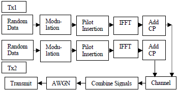
The following Figure 3 shows the MIMO transmitter system for two transmit antennas. The generated 3-dimensional random data symbols to allocate 3D-MIMO OFDM system are complex (integers) and a 4-ary modulation scheme is employed to modulate the data vector. 3D-scattered pilots are also complex numbers and are interleaved at odd position along the combined data-pilot vector comprising of 128 symbols including 64 data symbols as shown in the Figure 1 below.
Figure 1. 128 symbols after Interleaving of 64 Data symbols and 64 Pilot symbols
A guard band of 32 symbols is placed at the beginning of 128 symbols vector amounting to total 160 complex symbols. The 32 complex symbols for cyclic prefix are copied from the end of 128 data-pilot symbols. The numbers of symbols for cyclic prefix are considered to be the one-fourth of vector represented by data-pilots. The arrangement for the same is depicted in Figure 2 below. The last 32 symbols from the 128 symbols represented by the data-pilots are copied at the beginning. The arrow in the figure indicates the similarity of the symbols.
Figure 2. 160 symbols after adding cyclic prefix at the beginning of data-pilot vector
Figure 3. MIMO system transmission with two transmitters
After adding the Cyclic Prefix (CP), the signals are convolved with the channel parameters h11, h12 and h21, h22 using the Y=XH standard form. The following equations were used for the channel coefficient multiplication.
$\mathrm{Y} 1=\mathrm{X} 1 * \mathrm{H} 11+\mathrm{X} 2 * \mathrm{H} 12$ (1)
$\mathrm{Y} 2=\mathrm{X} 1 * \mathrm{H} 21+\mathrm{X} 2 * \mathrm{H} 22$ (2)
Further the signals were combined for transmission. The final vector of 320 symbols: 160 of Y1 and 160 of Y2 were concatenated and then contaminated with additive white Gaussian noise.
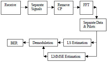
At the receiver, the signals are separated and the guard band is removed. The first 160 symbols correspond to transmitter 1 and remaining 160 for transmitter 2. The first 32 symbols from both vectors are discarded owing to cyclic prefix. Both the signals containing 128 remaining symbols of data-pilot arrangement were undergone through fast Fourier transform. The data-pilots were de-interleaved and separated for channel estimation. Figure 4 shows the operation performed at the receiver.
Figure 4. The receiver stages
Thus, at this stage, we have 64 symbols for each data and pilots for both the receiver. We carried the LS and the LMMSE Estimation using the following set of equations.
Let us consider the following notations: PT – transmitted pilots, PR-received pilots, DR- received data vector, then for LS estimation [17].
$\mathrm{t} 1=\mathrm{PT}^{\prime} * \mathrm{PT}$
$\mathrm{t} 2=$ inverse $(\mathrm{t} 1)$
$\mathrm{t} 3=\mathrm{PR}^{\prime} * \mathrm{PT}$
Channel Estimate HLS $=\mathbf{t} 2 * \mathbf{t} 3$ (3)
Estimated Data DE $1=$ inverse $(\mathrm{HLS}) * \mathrm{DR}$ (4)
Similarly, for LMMSE estimation [18]
$\mathrm{t} 1=\left(\mathrm{PT}^{\prime} * \mathrm{PT}\right) \cdot /(\mathrm{NR} * \mathrm{SIGMA})$
$\mathrm{t} 2=\mathrm{EYE}(\mathrm{NT}) \cdot /(\mathrm{NR} * \mathrm{SIGMAH})$
$\mathrm{t} 3=\text { inverse }(\mathrm{t} 1+\mathrm{t} 2)$
$\mathrm{t} 4=\left(\mathrm{PT}^{\prime} * \mathrm{PR}\right) \cdot /(\mathrm{NR} * \mathrm{SIGMA})$
Channel Estimate HLMMSE $=\mathbf{t} 3 * \mathbf{t} 4$ (5)
Estimated Data DE2 $=(\mathrm{DR} * \text { inverse (HLMMSE) })^{\prime}$ (6)
where, SIGMAH is a constant and the value considered in this work is 0.25. SIGMA is given by the following equation:
$\mathrm{SIGMA}=10^{(\mathrm{SNR} / 10)}$ (7)
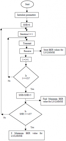
And the value of signal to noise ratio (SNR) in decibels (dB) range in [0:5:40]. Both the estimated data vectors are then demodulated. Each value of SNR is iterated 20 times and the minimum value of bit error rate (BER) is stored for LS and LMMSE estimation. The following Figure 5 shows the iterative loop with no optimization for LS and LMMSE. Here we have considered only one received signal that is signal 1 for estimation, demodulation and obtaining BER considering that signal 2 will give the same response.
Figure 5. Complete LS/LMMSE estimation system without optimization
The velocity a particle acquires and the position it must take in the search space during each step are governed by the following equations:
$\begin{aligned} \mathrm{VN}[]=\mathrm{W} * \mathrm{V}[] &+\mathrm{C} 1 * \mathrm{RAND}() *(\mathrm{PBEST}[]-\mathrm{P}[])+\mathrm{C} 2 * \mathrm{RAND}()(\mathrm{GBEST}[]-\mathrm{P}[]) \end{aligned}$ (8)
$\mathrm{PN}[]=\mathrm{P}[]+\mathrm{VN}[]$ (9)
where, PN and VN are the new position and the velocity of the particle. W is the inertial weight factor and used to govern the percentage of last velocity a particle should acquire in the current iteration. The inertia weight controls the amount of recurrence in the particle's velocity so that no two particles moving in the search area are at the same place at any instant [19]. The first term in the velocity equation is also termed as Retarding velocity.
PBEST[ ] is the particle best position from all the last positions it acquired from initial position to the current position. P[ ] is the particle current position. The second term in the velocity equation represents particle local statistics.
GBEST[ ] is the best position of a particle in the swarm among all particles in the current iteration. The third term in the velocity equation represents the global statistic (Communication with Neighborhood).
RAND( ) is the stochastic variable in the range [0 1] and can be considered same for term 2 and term 3 or may be different. C1 and C2 (learning factors) are constants being initialized with proper values at the beginning. In most of the research, a value of 2 is considered for both constant. The new position of a particle is given by the second equation above involves addition of the new velocity with the current position. Thus, the particle irrespective of the fitness takes the new position in the space subjected to some search space boundary conditions such as limiting the position and velocity to full dynamic range and distance a particle would travel in one step.
Initially all the particles (Swarm agents) are randomly positioned in the search place with some initial velocities. As the agents propagates, they acquire new position and velocities as per the equation stated above. The search space may be small or wide depending upon the complexity of the problem. Here we are interested to find value of (optimized) H (for LS and LMMSE) so that the bit error rate would be less than that obtained from standard LS and LMMSE estimation. From Figure 5, we have the last output as the minimum BER values for LS and LMMSE for each SNR value.
Table 1. Initial parameter settings for PSO
|
Sr.No. |
PSO Parameter |
Reference |
Value/Type |
|
1. |
Number of Particles in Swarm |
Number of iterations for each SNR value |
20 |
|
2. |
Initial particles position |
H values obtained by LMMSE corresponding to 20 iterations |
Complex |
|
3. |
Initial particles velocity |
Random complex numbers |
Random & Complex |
|
4. |
Initial PBEST values |
H values obtained by LMMSE corresponding to 20 iterations |
Complex |
|
5. |
Initial GBEST value |
Minimum H obtained by comparing H of LS and H of LMMSE |
Complex |
|
6. |
Number of epochs for PSO |
- |
100
|
|
7. |
Minimum particle position limit |
- |
0
|
|
8. |
Maximum particle position limit |
- |
3√2
|
|
9. |
Minimum velocity limit |
- |
0
|
|
10. |
Maximum velocity limit |
- |
25√2
|
|
11. |
Error Tolerance |
- |
0 |
Hence by simply comparing the BER values of LS and LMMSE, we obtained the minimum BER value for each SNR value. The respective channel estimate H (either for LS or LMMSE) corresponding to this minimum BER is also obtained. The following Table 1 shows the initialization of various PSO parameters.
In Table 1 the reason why initial position of particles is initialized to the H values obtained by LMMSE is that LMMSE has better performance over LS and is proved in literature. The PSO will iterate for searching new value for H for which the BER will be less than that obtained earlier after comparing BER obtained by LS and LMMSE estimation. Since any optimization technique is an approximation, it may happen that in some cases PSO will not be able to find a better solution as compared to the minimum BER obtained using LS/LMMSE estimation due to parameter constraints. In those cases, the earlier value is considered.
Figure 6. Optimized LS/LMMSE based Channel Estimation Algorithm using PSO
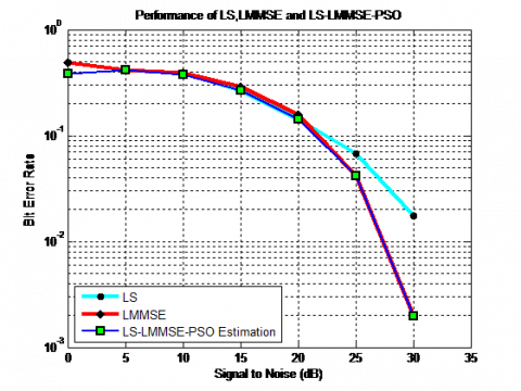
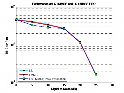
The novelty of the work lies in how the optimization is incorporated. The Figure 7 below shows the optimized performance obtained using PSO. The performance is plotted for signal to noise ration v/s bit error rate. Line in Green color indicates the performance obtained using PSO. After obtaining the channel estimate using PSO, the data vector is estimated again, demodulated and BER is found. The graphs in the figure clearly shows that LS performs better at higher SNR and LMMSE performs better at low SNR values. The PSO optimized BER scales down as compared to the other two standard estimation techniques.
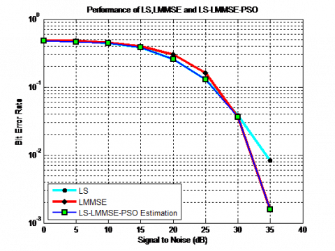
In Figure 8, the performance of PSO is better at higher SNR while LS and LMMSE performance carry their usual characteristics. In Figure 9, LS and LMMSE shows similar performance, but PSO performs better at higher SNR values.
Figure 10 is the typical situation where PSO is unable to perform better than LS or LMMSE. A stated earlier, it follows the best of LS and LMMSE estimation. The optimization was applied to small but realistic model of 2x2 MIMO where all the parameters were considered to be of complex numbers. This was considered owing to the computational and time complexity for higher MIMO systems.
Figure 7. Performance of PSO optimization over LS/LMMSE estimation techniques in 2x2 MIMO systems
Figure 8. Better Performance of PSO optimization at higher SNR
Figure 9. Better Performance of PSO optimization at higher SNR in case where LS and LMMSE shows similarity
Figure 10. Performance of PSO optimization follows best of LS and LMMSE estimation
Also, a simpler version of PSO [20] was used for optimization. Tuning of parameters of PSO was a challenging task for such complex environment. Proper and fine tuning of parameters can produce good optimization. A good and robust PSO variant with local and global search mechanism would have perform better. We had used only 20 agents in the search space. Increasing number of agents up to 40 can search the target early with some permissible error tolerance value (here tolerance is set to 0). The initial position of the particles was initialized with H of LMMSE obtained after the last 20th iteration but not considered the H for the best BER obtained with LMMSE. This had initially placed the particle somewhat away from the target in the search place with utmost 100 steps to achieve it. Similar approach was used by Vidhya and Shankar Kumar [21] where the channel parameters were fine-tuned using PSO and GA. They showed that such fine tuning produced better results than LS/MMSE estimation. Researchers [15] used GA in Massive MIMO with Rayleigh fading channel for obtaining best channel matrix to minimize mean squared error with low complexity. They showed that GA-MMSE works well at low SNR, GA-LMMSE at high SNR and GA-LS performance was better than MMSE. Latest work [16] used PSO with new cost function to reduce the computational complexity of Maximum Likelihood detector and verified by implementing the system on FPGA.
[1] Kennedy, J., Eberhart, R.C., Shi, Y. (2004). Swarm Intelligence. Morgan Kaufmann Publishers, San Francisco, CA.
[2] Kennedy, J., Eberhart, R.C. (1995). Particle swarm optimization. In Proceedings of the 1995 IEEE International Conference on Neural Networks, 4: 1942-1948. http://dx.doi.org/10.1109/ICNN.1995.488968
[3] Almamori, A., Mohan, S. (2018). Improved MMSE channel estimation in massive MIMO system with a method for the prediction of channel correlation matrix. 2018 IEEE 8th Annual Computing and Communication Workshop and Conference (CCWC), Las Vegas, NV, pp. 670-672. https://doi.org/10.1109/ccwc.2018.8301699
[4] Lv, C., Duan, J., Yang, Z. (2018). Two–stage channel estimation assisted by correlation exploitation for amplify and forward relay networks with multiple transmit and receive antennas. Progress in Electromagnetics Research M, 75: 13-20. http://dx.doi.org/10.2528/PIERM18080301
[5] Bangash, K., Khan, I., Lloret, J., Leon, A. (2018). A joint approach for low – complexity channel estimation in 5G massive MIMO systems. Electronics 2018, 7(10): 218. http://dx.doi.org/10.3390/electronics7100218
[6] Fang, T., Zeng, G. (2018). A new pilot–based block low–rank channel estimation algorithm for massive MIMO. Proceedings of the 2018 2nd International Conference on Algorithms, Computing and Systems, pp. 200-204. http://dx.doi.org/10.1145/3242840.3242886
[7] Jing, X., Li, M., Liu, H., Li, S., Pan, G. (2018). Superimposed pilot optimization design and channel estimation for multiuser massive MIMO systems. IEEE Transactions on Vehicular Technology, 67(12): 11818-11832. http://dx.doi.org/10.1109/TVT.2018.2875480
[8] Ma, X., Yang, F., Cheng, L., Song, J. (2018). Sparse channel estimation for MIMO systems based on time –domain training sequence optimization. 2018 14th International Wireless Communications & Mobile Computing Conference (IWCMC), Limassol, pp. 406-411. http://dx.doi.org/10.1109/IWCMC.2018.8450484
[9] Sumitra, N., Motade, Kulkarni, A.V. (2018). Channel estimation and estimation and data detection using machine learning for MIMO 5G communication systems in fading channel. Technologies 2018, 6(3): 72. https://doi.org/10.3390/technologies6030072
[10] Soleimani, H., De Donno, D., Tomasin, S. (2018). Mm-Wave channel estimation with accelerated gradient descent algorithms. EURASIP Journal on Wireless Communications and Networking, 2018(1). http://dx.doi.org/10.1186/s13638-018-1282-3
[11] Lv, Z., Yang, T., Zhu, C. (2018). Channel estimation and pilot design for massive MIMO systems with block–structured compressive sensing. IOP Conference Series: Materials Science and Engineering, 322(5): 052039. http://dx.doi.org/10.1088/1757-899X/322/5/052039
[12] Biguesh, M., Gershman, A.B. (2006). Training–based MIMO channel estimation: A study of estimator tradeoffs and optimal training signals. IEEE Transactions on Signal Processing, 54(3): 884-893. http://dx.doi.org/10.1109/TSP.2005.863008
[13] Dai, J., Liu, A., So, H.C. (2019). Non–uniform burst–sparsity learning for massive MIMO channel estimation. IEEE Transactions on Signal Processing, 67(4): 1075-1087. http://dx.doi.org/10.1109/TSP.2018.2889952
[14] Waseem, A., Naveed, A., Ali, S., Arshad, M., Anis, H., Qureshi, I.M. (2019). Compressive sensing based channel estimation for massive MIMO communication systems. Wireless Communications and Mobile Computing, Hindawi, 2019: 15 pages. http://dx.doi.org/10.1155/2019/6374764
[15] Noman, M.K., Islam, S.M.S., Hasan, S., Parveen, R. (2019). An improved data aided channel estimation technique using genetic algorithm for massive MIMO. International Conference on Machine Learning and Data Engineering, Sydney, Australia, pp. 61-66. http://dx.doi.org/10.1109/iCMLDE.2018.00022
[16] Trimeche, A., Sakly, A., Mtibaa, A. (2017). Implementation of PSO algorithm for MIMO detection system in FPGA. International Journal of Electronics, 105(1): 42-57. http://dx.doi.org/10.1080/00207217.2017.1335801
[17] Su, W., Pan, Z.W. (2007). Iterative LS channel estimation for OFDM systems based on transform-domain processing. 2007 International Conference on Wireless Communications, Networking and Mobile Computing, Shanghai, pp. 416-419. http://dx.doi.org/10.1109/WICOM.2007.110
[18] Carlos, R., Atilio, G. (2008). An OFDM symbol design for reduced complexity MMSE channel estimation. Journal of Communications, 3(4). https://doi.org/10.4304/jcm.3.4.26-33
[19] Eberhart, R.C., Shi, Y. (2000). Comparing inertia weights and constriction factors in particle swarm Optimization. Proceedings of the 2000 Congress on Evolutionary Computation, CA, USA, 1: 84-88. http://dx.doi.org/10.1109/CEC.2000.870279
[20] Chen, W.N., Zhang, J., Chung, H.S.H. (2010). A novel set–based particle swarm optimization method for discrete optimization problems. IEEE Transactions on Evolutionary Computation, 14(2): 278-300. https://doi.org/10.1109/tevc.2009.2030331
[21] Vidhya, K., Shankar Kumar, K.R. (2014). Channel Estimation of MIMO-OFDM system using PSO and GA. Arabian Journal of Science and Engineering, 39(5): 4047-4056. http://dx.doi.org/10.1007/s13369-014-0988-8