Salim Ouchtati* | Abdelhakim Chergui | Sébastien Mavromatis | Belmeguenai Aissa | Djemili Rafik | Jean Sequeira
© 2019 IIETA. This article is published by IIETA and is licensed under the CC BY 4.0 license (http://creativecommons.org/licenses/by/4.0/).
OPEN ACCESS
In this paper, a novel system is proposed for automating the process of brain tumor classification in magnetic resonance (MR) images. The proposed system has been validated on a database composed of 90 brain MR images belonging to different persons with several types of tumors. The images were arranged into 6 classes of brain tumors with 15 samples for each class. Each MR image of the brain is represented by a feature vector composed of several parameters extracted by two methods: the image entropy and the seven Hu's invariant moments. These two methods are applied on selected zones obtained by sliding a window along the MR image of the brain. The size of the used sliding window is 16x16 pixels for the first method (image entropy) and 64x64 pixels for the second method (seven Hu’s invariant moments). To implement the classification, a multilayer perceptron trained with the gradient backpropagation algorithm has been used. The obtained results are very encouraging; the resulting system properly classifies 97.77% of the images of the used database.
artificial neural networks, medical images processing, images classification, brain tumor
Computer-aided diagnosis and medical image processing are efficient tools for solving a large number of problems in medicine and have made significant advances in the preceding decade [1-5]. The two research areas are among the most important and offer new ideas and improve diagnostic procedures and treatment decisions for large varieties of diseases and abnormalities, particularly brain tumors. Presently, the use of the medical image processing to study this type of abnormality is not an easy task. Many studies have been performed to detect the existence of brain tumors, their nature and their exact locations [6], and most of these studies are based on the use of the powerful tool of magnetic resonance (MR) imaging of the brain [6-10]. This imaging type is generally used in medicine to collect and visualize details of the internal body structure. The amount of information contained in an MR image is extremely large compared to all other types of imaging, and MR imaging is becoming a very efficient tool for the diagnosis of several diseases, especially when dealing with brain tumor detection and cancer imaging, and the ideal method for evaluating the patients having signs of brain tumors. The high performance of MR imaging arises from this technique being characterized by a multiplanar capability, a superior contrast and a high image resolution that allows it to efficiently assess tumor location.
In order to improve the results obtained in the study that we presented in the 2nd International Conference on Advanced Systems and Electrical Technologies (IC_ASET'2018) [10], we propose a novel system of detection and classification of brain tumors. In the study [10], the feature vector used to represent the MR image of the brain is composed of a set of parameters extracted using the central moments of order 1, 2 and 3 of histograms of zones obtained after sliding a window of size 16x16 pixel on the MR image of the brain, while the parameters of the feature vector used in this study is based on the calculation of the entropy and the seven Hu’s invariant moments of each zone selected by sliding a window along the brain image. Note that for some reasons that depend on the computation time and the available memory space, the size of the used sliding window is not the same for both methods. On this basis, the sliding window used for entropy calculation is 16x16 pixels, while the size of that used for the calculation of Hu’s invariant moments is 64x64 pixels. We will explain the reasons that prompted us to change the size of the sliding window for calculation of Hu’s invariant moments in detail in one of the following paragraphs of this paper. The classification is achieved by a multilayer perceptron trained with the gradient backpropagation algorithm. The proposed system has been validated on a database composed of a set of brain MR images belonging to different persons with several types of tumors. The proposed system can produce four different answers: a recognized brain tumor, an ambiguous brain tumor, a rejected brain tumor and a wrong brain tumor. Therefore, for the evaluation of the proposed system the following rates were calculated: Recognition Rate (R_R), Ambiguity Rate (A_R), Rejection Rate (RJ_R) and Error Rate (E_R). The values of various rates clearly show that the obtained results are very encouraging and very promising; the system is able to properly classify 97.77% of brain images of the used database.
This paper is organized as follows: the next section presents some related studies in the field of brain tumors classification. The database used to validate the proposed method is described in section 3. The different parts of the proposed system and the used methodology are exposed in section 4. The obtained results of this study are shown in section 5. Finally, the most relevant conclusions are recorded in section 6.
Ruan et al. [11] proposes a method based on the use of partial volume modeling for brain tissue classification in MR images. The researchers consider two classes in a brain dataset. The first is called the pure class, and is composed of the three main types of brain tissue: gray matter, white matter, and cerebrospinal fluid. The second is called mixed class, and is composed mainly of mixtures. The proposed method proceeds in two steps, both of which are based on the use of Markov Random Field (MRF) models. The first step consists of segmenting the brain into pure classes and mixed class, while the second consists of reclassifying mixed class into pure classes using some knowledge of the obtained pure classes. This method has been evaluated on simulated and real-world brain MR images.
The method proposed by Bauer et al. [12] has been tested on the BRATS2012 database [13] composed of simulated and clinical images. The main objective of this method is not only to separate healthy tissues from the pathologic tissue but also, on one hand, to classify healthy tissues into three components: gray matter (GM), white matter (WM) and cerebrospinal fluid (CSF), and on the other hand, to classify pathologic tissue into the following components: necrotic, active and edema. According to the authors, convincing results have been obtained (the average Dice coefficient equal to 0.73 for tumor and 0.59 for edema) within an acceptable computation time (approximately 4 to 12 minutes).
Cobzas et al. [14] propose a variational segmentation algorithm for brain tumors by using a high-dimensional feature set calculated from MRI data and registered atlases. The learning of the statistical model for tumor and normal tissue is implemented by using manually segmented data. According to the authors, the use of the conditional model to discriminate between normal and abnormal regions significantly improves the segmentation results compared to those of the traditional generative models.
The objective of the study proposed by Iftekharuddin et al. [15] is to develop a new technique for brain tumor segmentation. The authors use information extracted from the multiresolution texture data that combines fractal Brownian motion (fBm) and wavelet multiresolution analysis, and the proposed technique has been evaluated on pediatric brain MR images from St. Jude Children’s Research Hospital. Both the pixel intensity and the multiresolution texture features are exploited to obtain a segmented tumor. In the next step, the presence of tumor in an MR brain image is statistically validated by using the feedforward (FF) neural network as a classifier.
The main objective of the study proposed by Zhang et al. [16] is the development of an accurate system for detection of brain pathologies from MR images of the brain. The proposed method is based on the use of entropy of the wavelet and the Hu’s moment invariants for feature extraction, while the classification is performed first by the generalized eigenvalue proximal support vector machine (GEPSVM); afterwards, to improve the results of classification, the authors use the popular radial basis function (RBF) kernel. According to the authors of this study, the results obtained show that the proposed method is effective and can be used in real-world applications.
In the context of brain tumor classification, Chaplot et al. [17] have proposed a new method of classifying brain MR images for either normal or abnormal cases. The study is based on the comparison of results obtained by using the classifiers in two steps: first, neural network self-organizing maps and second, the support vector machine. Note that the authors have used wavelets for the input of the two classifiers. The proposed method has been tested on fifty-two brain MR images; according to the authors, the obtained results are very encouraging, and the classification rate of the support vector machine classifier is observed to be higher than that obtained by using the self-organizing maps classifier.
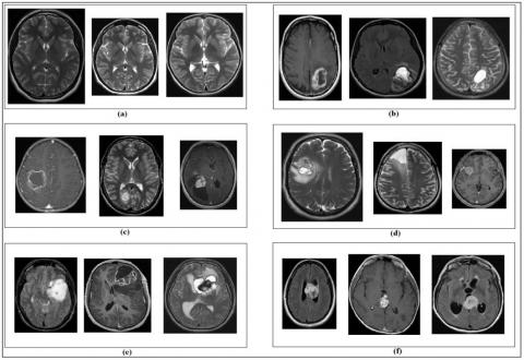
To validate the proposed method, we have used a set of clinical MR images extracted from the “Radiopaedia” website [18]. According to the absence or presence of a tumor and its location in the brain, the MR images are arranged in six (6) classes with fifteen (15) different samples for each class. These classes are defined as follows:
Figure 1 shows brain MR images of several samples of each class of the used database
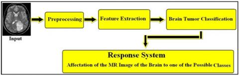
The proposed system is composed of three essential steps (see Figure 2), namely, preprocessing, feature extraction and brain tumor classification. The role of and various methods and techniques used for each step are described as follows:
4.1 Preprocessing
The only preprocessing operation we consider necessary in this study is image resizing; this operation is performed due to the nature of the feature extraction methods in the next step that are only applied to normalized images. As brain images have variable sizes, the preprocessing step consists of resizing all images of the database to all images of the database to 128x128 pixels in size. Note that the choice of the size 128x128 pixels as a normalized size for the images of the used database is related to the nature of the feature extraction methods used in this study. Resizing MR images to a size of 128x128 pixels allows us to obtain an appropriate number of zones selected by the sliding window used for each method.
Figure 1. Several samples of each class of the used database: a) Samples of class 01, b) Samples of class 02, c) Samples of class 03, d) Samples of class 04, e) Samples of class 05, f) Samples of class 06
Figure 2. General schema of the proposed system
4.2 Feature extraction
In this paper, the feature vector is composed of several parameters extracted from the brain MR image by two methods, the first based on the calculation of image entropy, and the second consisting of the calculation of the seven Hu’s invariant moments; the both methods are applied on each zone selected by sliding a window over the brain MR image. For reasons involving computation time and required memory, the sizes of the sliding windows used for the two methods are not the same; the size of the sliding window used for the entropy method is 16x16 pixels, while the size used for Hu’s invariant moments method is 64x64 pixels. Note that we have used sample 01 of class 02 and sample 03 of class 03 as examples to explain the principle of these two methods and to show the obtained features or parameters.
As it was requested in paper [18], the sources of these two samples are as follows:
4.2.1 Image entropy
The notion of entropy has been widely used for brain pathology classification [16, 19-23] and can be defined as the concept of the spread of states a system can be in. A system that occupies a small number of such states is characterized by low entropy, while a system that occupies a large number of states is characterized by high entropy.
In the case of an image, interpreting the preceding entropy definition leads us to consider the states as the grayscale levels an individual pixel can have. In particular, there are 256 states for a grayscale image when the pixels are represented using 8 bits.
The entropy of the image reaches the maximum value if the spread of the states is maximized, this holds if all such states are equally occupied, as they are in an image that has been perfectly histogram-equalized. On the other hand, if the image has been processed using a threshold, then only two states are occupied, and consequently the entropy is low. If all the pixels have the same value, the entropy of the image is zero. In conclusion, the entropy of an image varies proportionally to its information content. The entropy changes from high entropy of a full grayscale image to low entropy of a threshold binary image and to zero entropy of a single-valued image.
The entropy E of an image is defined as
$E=-\sum\limits_{k=0}^{M-1}{{{P}_{k}}{{\log }_{2}}({{P}_{k}})}$ (1)
where, M is the number of grayscale levels, and Pk is the probability associated with grayscale level k.
4.2.2 Seven Hu’s invariant moments
Invariant moments have been widely applied to image processing [16, 22] and have proven useful in a variety of applications due to their invariance with respect to image translation, scaling and rotation. They were first introduced by Hu [24], who derived six absolute orthogonal invariants and one skew orthogonal invariant based upon algebraic invariants, which are independent not only of position, size and orientation but also of parallel projection. Invariant moments have been proven to be the adequate measures for tracing image patterns affected by image translation, scaling and rotation under the assumption of noise-free images with continuous functions. The quantities used to construct the invariant moments are defined in the continuous form, but for practical implementation they are computed in the discrete form. For a two-dimensional continuous function f(x,y), the moment (sometimes called the "raw moment") of order (p +q) is defined as
${{M}_{pq}}=\int_{-\infty }^{\infty }{\int_{-\infty }^{\infty }{{{x}^{p}}{{y}^{d}}f(x,y)dxdy}}$ (2)
Mpq is a two-dimensional moment of function f(x,y), where the indices p and q are both natural numbers. Adapting this to a grayscale image with pixel intensities I(x,y), the raw moments Mpq become
${{M}_{pq}}=\sum\limits_{x}{\sum\limits_{y}{{{x}^{p}}{{y}^{q}}I(x,y)}}$ (3)
One should note that the Mpq moments are not invariant with respect to f(x,y) changing by translation, rotation and scaling. The moment that is invariant to translation can be obtained by calculating the moment of order (p+q) called central moment and given by the following equation:
${{\mu }_{pq}}=\int_{-\infty }^{\infty }{\int_{-\infty }^{\infty }{{{\left( x-\overline{x} \right)}^{p}}{{\left( y-\overline{y} \right)}^{q}}f(x,y)dxdy}}$ (4)
where, $\bar{x}$ and $\cdot \bar{y}$ are the coordinates of the gravity center of the image, calculated using Eq. (3) and given by
$\overline{x}=\frac{{{M}_{10}}}{{{M}_{00}}}\begin{matrix} {} & {} \\\end{matrix}\overline{y}=\frac{{{M}_{01}}}{{{M}_{00}}}$ (5)
In the case of a grayscale image with intensity I(x,y), Eq. (4) becomes
${{\mu }_{pq}}=\sum\limits_{x}{\sum\limits_{y}{{{\left( x-\overline{x} \right)}^{p}}{{\left( y-\overline{y} \right)}^{q}}I(x,y)}}$ (6)
The central moments can be extended to be both translation- and scale-invariant by using the following equation:
${{\eta }_{pq}}=\frac{{{\mu }_{pq}}}{\mu _{00}^{\left( 1+\frac{p+q}{2} \right)}}$ (7)
The obtained moments are called the normalized central moments. To enable rotation invariance, based on the above moments (normalized central moments), Hu introduced the seven invariant moments given by the following equations:
${{\Phi }_{1}}={{\eta }_{20}}+{{\eta }_{02}}$ (8)
${{\Phi }_{2}}={{\left( {{\eta }_{20}}-{{\eta }_{02}} \right)}^{2}}+4\eta _{11}^{2}$ (9)
${{\Phi }_{3}}={{\left( {{\eta }_{30}}-3{{\eta }_{12}} \right)}^{2}}+{{\left( 3{{\eta }_{21}}-{{\eta }_{03}} \right)}^{2}}$ (10)
${{\Phi }_{4}}={{\left( {{\eta }_{30}}+{{\eta }_{12}} \right)}^{2}}+{{\left( {{\eta }_{21}}+{{\eta }_{03}} \right)}^{2}}$ (11)
$\begin{align} & {{\Phi }_{5}}=\left( {{\eta }_{30}}-3{{\eta }_{12}} \right)\left( {{\eta }_{30}}+{{\eta }_{12}} \right)\left[ {{\left( {{\eta }_{30}}+{{\eta }_{12}} \right)}^{2}}-3{{\left( {{\eta }_{21}}+{{\eta }_{03}} \right)}^{2}} \right] \\ & \begin{matrix} {} \\\end{matrix}+\left( 3{{\eta }_{21}}-{{\eta }_{03}} \right)\left( {{\eta }_{21}}+{{\eta }_{03}} \right)\left[ 3{{\left( {{\eta }_{30}}+{{\eta }_{12}} \right)}^{2}}-{{\left( {{\eta }_{21}}+{{\eta }_{03}} \right)}^{2}} \right] \\ \end{align}$ (12)
$\begin{align} & {{\Phi }_{6}}=\left( {{\eta }_{20}}-{{\eta }_{02}} \right)\left[ {{\left( {{\eta }_{30}}+{{\eta }_{12}} \right)}^{2}}-{{\left( {{\eta }_{21}}+{{\eta }_{03}} \right)}^{2}} \right] \\ & \begin{matrix} {} & {} \\\end{matrix}+4{{\eta }_{11}}\left( {{\eta }_{30}}-{{\eta }_{12}} \right)\left( {{\eta }_{21}}+{{\eta }_{03}} \right) \\ \end{align}$ (13)
$\begin{align} & {{\Phi }_{7}}=\left( 3{{\eta }_{21}}-{{\eta }_{03}} \right)\left( {{\eta }_{30}}+{{\eta }_{12}} \right)\left[ {{\left( {{\eta }_{30}}+{{\eta }_{12}} \right)}^{2}}-3{{\left( {{\eta }_{21}}+{{\eta }_{03}} \right)}^{2}} \right] \\ & \begin{matrix} {} \\\end{matrix}+\left( {{\eta }_{30}}-3{{\eta }_{21}} \right)\left( {{\eta }_{21}}+{{\eta }_{03}} \right)\left[ 3{{\left( {{\eta }_{30}}+{{\eta }_{12}} \right)}^{2}}-{{\left( {{\eta }_{21}}+{{\eta }_{03}} \right)}^{2}} \right] \\ \end{align}$ (14)
4.3 Brain tumor classification
In this study, the classification is achieved using a neural network composed of three layers; namely, the input layer whose number of neurons is equal to the size of the used feature vector (N_IL=92); the output layer whose number of neurons is equal to the number of brain tumor classes to be recognized (N_OL=6), and one hidden layers whose number of neurons is experimentally chosen equal to fifty-five (55) (N_HL=55). The initial connection weights are randomly chosen in the range of [-1, 1]. The transfer function used is the familiar sigmoid function. The large use of the back propagation training method for a great number of pattern recognition problems and its simplicity encouraged us to use it for training the neural network. The principle of this method is based on the gradient descent algorithm, the learning rate is experimentally chosen and it allows the algorithm to converge more easily if it is properly chosen by the experimenter. In our case, we have opted for a rate η= 0.8.
5.1 Entropy values
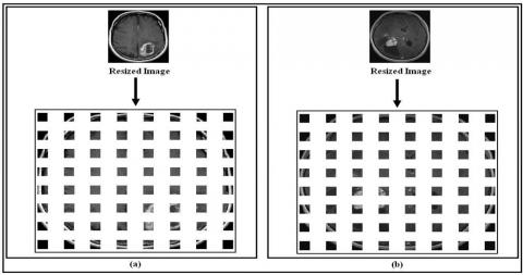
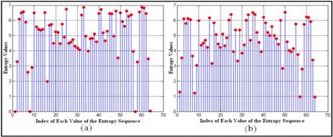
In this study, the image entropy is one of methods we have used to characterize brain images; the method consists of calculating the entropy only for selected zones of a brain image instead of the entire image. The principle is to slide a window of size 16x16 pixels along the brain MR image and to calculate the entropy for each selected zone using equation (1). Since the size of the brain image is 128x128 pixels, this method allows us to obtain 64 (sixty-four) zones, and therefore 64 (sixty-four) values of entropy. Figure 3 shows sixty-four zones obtained after sliding a window of size 16x16 pixels over sample 01 of class 02 and sample 03 of class 03, while entropy values (E) for each zone (Z) for the same samples are shown in a graphical form in Figure 4 and in the numeric form in Table 1 and Table 2.
Figure 3. Sixty-four zones obtained after sliding a window of size 16x16 pixels over the MR image: (a) sample 01 of class 02; (b) sample 03 of class 03
Figure 4. Entropy values of sixty-four zones: (a) sample 01 of class 02; (b) sample 03 of class 03
Table 1. Numeric values of entropy of sixty-four zones for sample 01 of class 02
|
Z |
E |
Z |
E |
Z |
E |
Z |
E |
|
01 |
0 |
17 |
5.682 |
33 |
6.876 |
49 |
3.521 |
|
02 |
3.275 |
18 |
5.747 |
34 |
4.973 |
50 |
6.503 |
|
03 |
6.097 |
19 |
4.489 |
35 |
3.976 |
51 |
5.929 |
|
04 |
6.499 |
20 |
5.247 |
36 |
4.805 |
52 |
5.611 |
|
05 |
6.580 |
21 |
5.216 |
37 |
4.825 |
53 |
6.631 |
|
06 |
5.891 |
22 |
4.468 |
38 |
5.115 |
54 |
6.266 |
|
07 |
2.579 |
23 |
5.768 |
39 |
4.603 |
55 |
6.381 |
|
08 |
0 |
24 |
4.908 |
40 |
6.466 |
56 |
3.960 |
|
09 |
2.886 |
25 |
6.739 |
41 |
6.725 |
57 |
0 |
|
10 |
6.508 |
26 |
4.482 |
42 |
5.194 |
58 |
3.267 |
|
11 |
5.569 |
27 |
4.571 |
43 |
4.655 |
59 |
6.555 |
|
12 |
5.422 |
28 |
4.744 |
44 |
5.297 |
60 |
6.875 |
|
13 |
5.356 |
29 |
4.318 |
45 |
6.466 |
61 |
6.816 |
|
14 |
5.418 |
30 |
4.181 |
46 |
6.441 |
62 |
6.450 |
|
15 |
6.518 |
31 |
4.071 |
47 |
4.960 |
63 |
3.474 |
|
16 |
1.979 |
32 |
6.359 |
48 |
6.617 |
64 |
0.036 |
Table 2. Numeric values of entropy of sixty-four zones for sample 03 of class 03
|
Z |
E |
Z |
E |
Z |
E |
Z |
E |
|
01 |
1.286 |
17 |
5.841 |
33 |
6.369 |
49 |
2.838 |
|
02 |
3.529 |
18 |
5.062 |
34 |
4.702 |
50 |
6.541 |
|
03 |
6.101 |
19 |
4.461 |
35 |
6.518 |
51 |
4.591 |
|
04 |
5.810 |
20 |
4.218 |
36 |
6.390 |
52 |
4.032 |
|
05 |
6.135 |
21 |
5.099 |
37 |
5.210 |
53 |
3.934 |
|
06 |
6.042 |
22 |
4.319 |
38 |
4.550 |
54 |
4.150 |
|
07 |
3.663 |
23 |
4.852 |
39 |
3.947 |
55 |
5.754 |
|
08 |
1.223 |
24 |
6.033 |
40 |
6.213 |
56 |
3.754 |
|
09 |
3.031 |
25 |
6.405 |
41 |
5.852 |
57 |
0.971 |
|
10 |
5.996 |
26 |
3.945 |
42 |
5.207 |
58 |
2.788 |
|
11 |
4.378 |
27 |
5.367 |
43 |
5.008 |
59 |
5.750 |
|
12 |
4.508 |
28 |
3.334 |
44 |
5.599 |
60 |
6.241 |
|
13 |
4.699 |
29 |
5.376 |
45 |
4.995 |
61 |
6.196 |
|
14 |
4.230 |
30 |
3.840 |
46 |
4.799 |
62 |
5.924 |
|
15 |
6.179 |
31 |
4.395 |
47 |
4.436 |
63 |
3.388 |
|
16 |
3.171 |
32 |
6.007 |
48 |
6.008 |
64 |
0.950 |
5.2 Seven Hu’s invariant moments values
In this work, the seven Hu’s invariant moments are also used to characterize the brain image. The idea is to slide another window of size 64x64 pixels along the brain MR image and, for each selected zone, calculate the seven Hu’s invariant moments by using Eqns. (8-14), which will allow us to obtain twenty-eight (28) features. Note that the use of a window of size 16x16 pixels for the entropy calculation allows us to obtain sixty-four (64) parameters, while the use of the same window for the calculation of seven Hu’s invariant moments allow us to obtain four hundred and forty-eight (448) parameters. Comparatively, this is indeed a large number, which will consequently increase the computation time and reduce available memory. This is the main reason for choosing a window size of 64x64 pixels instead of 16x16 pixels for Hu’s invariants moment calculation.
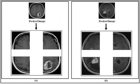
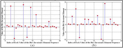
The four zones obtained after sliding a window of size 64x64 pixels on sample 01 of class 02 and sample 03 of class 03 are shown in Figure 5, while the values of the Hu’s invariant moments for the same samples are shown in a graphical form in Figure 6 and in the numeric form in Table 3 and Table 4.
5.3 Used feature vector
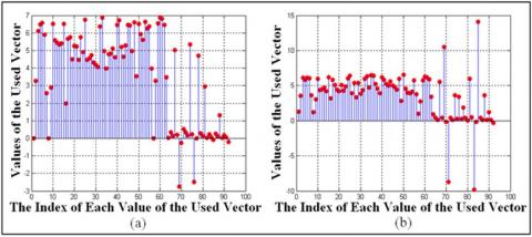
It is the features vector used to characterize the brain image, and with which, we will nourish the recognition module, its size is equal to ninety-two (92) parameters; it is composed of sixty four (64) parameters obtained by the image entropy method and twenty-eight (28) parameters obtained by Hu’s invariant moments method. The feature vectors of several samples of the used database are shown in a graphical form in Figure 7.
5.4 The learning step
The learning of the neural network was realized using only sixty (60) samples (ten samples of each class). The network learning process is stopped only when the sum of the mean square error reached a value equal to 0.0001. Figure 8 shows the evolution of the mean square error during the learning step.
5.5 The test step
During this phase, all samples of the database (i.e., ninety (90) samples) are successively presented at the system input, and for each sample the system makes a decision to assign it to one of the possible classes. The response of the system can be one of the following:
Figure 5. Four zones obtained after the application of the sliding window of size 64x64 pixels: (a) Sample 01 of class 02; (b) Sample 03 of class 03
Figure 6. Four zones obtained after the application of the sliding window of size 64x64 pixels: (a) Sample 01 of class 02; (b) Sample 03 of class 03
Figure 7. Feature vectors of several brain MR images: (a) Feature vector of sample 01 of class 02; (b) Feature vector of sample 03 of class 03
Figure 8. Evolution of the mean square error during the learning step: (a) after 1045 epochs, (b) after 1958 epochs, (c) after 6600 epochs, (e) reaching the desired value after 17402 epochs
Table 3. Numeric values of Hu’s invariant moments of the four zones: sample 01 of class 02
|
|
Zone1 |
Zone2 |
Zone3 |
Zone4 |
|
Ф1 |
0.3474 |
0.3476 |
0.3008 |
0.2563 |
|
Ф2 |
0.1326 |
0.1789 |
0.1468 |
0.1128 |
|
Ф3 |
5.0378 |
5.3441 |
2.9579 |
1.3022 |
|
Ф4 |
0.1916 |
0.2409 |
0.0316 |
0.0376 |
|
Ф5 |
-2.7579 |
-2.4828 |
0.2300 |
0.1816 |
|
Ф6 |
-0.2759 |
-0.0027 |
0.0640 |
0.0571 |
|
Ф7 |
0.5179 |
4.7159 |
-0.0994 |
-0.1963 |
Table 4. Numeric values of Hu’s invariant moments of the four zones: sample 03 of class 03
|
|
Zone1 |
Zone2 |
Zone3 |
Zone4 |
|
Ф1 |
0.4369 |
0.4038 |
0.3905 |
0.4142 |
|
Ф2 |
0.1019 |
0.0964 |
0.0382 |
0.1394 |
|
Ф3 |
5.5322 |
3.6032 |
5.9701 |
3.6256 |
|
Ф4 |
0.4032 |
0.2582 |
0.4730 |
0.0944 |
|
Ф5 |
10.4721 |
3.4144 |
-9.8067 |
1.2369 |
|
Ф6 |
-0.1780 |
0.2559 |
-0.1710 |
0.1470 |
|
Ф7 |
-8.7078 |
1.8764 |
14.0988 |
-0.3329 |
5.6 Obtained rates
It should be noted that the evaluation of the performance of the implemented system has been done using all samples of the database (i.e., ninety (90) samples), and according to the four types of possible responses of the proposed system, four types of rates can be defined, namely, Recognition Rate (R_R), Ambiguity Rate (A_R), Rejection Rate (RJ_R) and Error Rate (E_R). The system's response can take many forms, among the ninety (90) samples, it correctly associates eighty eight (88) samples to their classes, accordingly, the Recognition Rate is equivalent to 97.77%, for other samples, the system doesn’t take any wrong decision of classification, this means that the Error Rate is equal to 0%, but it proposes an assignment of one sample to more than one class, and it doesn’t make any classification decision for another sample, this means that the Ambiguous Rate and the Rejected Rate are both equivalent to 1.11%.
The different obtained rates as well as the comparison of the method used in this study to those that adopted in previous studies of the same field are respectively shown in Tables 5 and 6. The results presented in the two tables clearly show the importance of the proposed method compared to other methods in the same field, this importance lies in the following points:
The proposed method is the only method that considers the calculation of Rejection, Ambiguity and Error rates. The calculation of these rates is very important, it allows us to have an idea about the nature of difficulties encountered by the system to correctly classifies the brain MR image and consequently to propose the necessary solutions to improve the recognition rate.
The results of the proposed method are much better than those obtained by other methods adopted in previous studies, this is due to the technique of the sliding window that we used to extract the features from the brain image, this technique is completely novel and it allowed us to have features not from the whole brain image, but from multiple zones of it, therefore, the information provided by applying this technique is more consistent than that provided if the feature extraction was performed on the whole image of the brain.
Table 5. Obtained rates
|
Rate |
Value (%) |
|
Recognition rate (R_R) |
97.77 |
|
Ambiguity rate (A_R) |
1.11 |
|
Rejection rate (RJ_R) |
1.11 |
|
Error rate (E_R) |
0.00 |
Table 6. Comparison of the proposed method to those that adopted in previous studies.
|
Study |
Number of images |
Recognition rate (R_R) % |
|
[8] |
33 |
85 |
|
[8] |
57 |
96.6 |
|
[8] |
65 |
94.28 |
|
[10] |
60 |
88.333 |
|
[20] |
64 |
92.60 |
|
The proposed |
90 |
97.77 |
This study explores the subject of automating the process of detection and classification of brain tumors from brain MR images. The importance of this type of study is due to solutions they propose to overcome multiple difficulties that have thus far prevented the implementation of a universal system for detection and automatic classification of brain tumors, such difficulties being mainly due to variability in tumor size and location in the brain. This study proposes a novel method for the classification of brain tumors by interpreting brain MR images. The main objective was to improve the results obtained in the study that we presented in the 2nd International Conference on Advanced Systems and Electrical Technologies (IC_ASET'2018) [10]. The proposed method is completely novel and it based on using of a new feature vector composed of several parameters obtained by applying two methods: the calculation of image entropy and Hu’s seven invariant moments. The first method consists of the calculation of entropy of each zone selected by sliding window 16x16 pixels in size, while the second method consists of the calculation of Hu’s seven invariant moments of each zone selected by other sliding window 64x64 pixels in size. The obtained results are very encouraging and they are better than those obtained in the work [10]. The system correctly classifies 97.77% of images of the used database, achieving an attractive recognition rate that can encourage further research. The results can be further improved by analyzing the images that have given the system difficulties when assigning them to their proper classes. This analysis will allow the identification of the reasons for misclassification and thus the proposal of necessary solutions for each stage of the system.
This work is supported by the Ministry of Higher Education and Scientific Research – Algeria- (PRFU project, Grant number: A10N01UN210120180002).
[1] Charfi, S., El Ansari, M., Balasingham, I. (2019). Computer-aided diagnosis system for ulcer detection in wireless capsule endoscopy images. IET Image Processing, 13(6): 1023-1030. http://dx.doi.org/10.1049/iet-ipr.2018.6232
[2] Zhang, J., Xia, Y., Xia, Y., Fulham, M., Feng, D.D. (2018). Classification of medical images in the biomedical literature by jointly using deep and handcrafted visual features. IEEE Journal of Biomedical and Health Informatics, 22(5): 1521-1530. http://dx.doi.org/10.1109/JBHI.2017.2775662
[3] Mansour, R.F. (2017). Evolutionary computing enriched computer-aided diagnosis system for diabetic retinopathy: A survey. IEEE Reviews in Biomedical Engineering, 10: 334-349. http://dx.doi.org/10.1109/RBME.2017.2705064
[4] Elizabeth, D.S., Nehemiah, H.K., Retmin Raj, C.S., Kannan, R. (2012). Computer-aided diagnosis of lung cancer based on analysis of the significant slice of chest computed tomography image. IET Image Processing, 6(6): 697-705. http://dx.doi.org/10.1049/iet-ipr.2010.0521
[5] Duraisamy, S., Emperumal, S. (2017). Computer-aided mammogram diagnosis system using deep learning convolutional fully complex-valued relaxation neural network classifier. IET Computer Vision, 11(8): 656-662. http://dx.doi.org/10.1049/iet-cvi.2016.0425
[6] Kaur, T., Saini, B.S., Gupta, S. (2017). Quantitative metric for MR brain tumour grade classification using sample space density measure of analytic intrinsic mode function representation. IET Image Processing, 11(8): 620-632. http://dx.doi.org/10.1049/iet-ipr.2016.1103
[7] Kermi, A., Andjouh, K., Zidane, F. (2018). Fully automated brain tumour segmentation system in 3D-MRI using symmetry analysis of brain and level sets. IET Image Processing, 12(11): 1964-1971. http://dx.doi.org/10.1049/iet-ipr.2017.1124
[8] Anitha, V., Murugavalli, S. (2016). Brain tumour classification using two-tier classifier with adaptive segmentation technique. IET Computer Vision, 10(1): 9-17. http://dx.doi.org/10.1049/iet-cvi.2014.0193
[9] Mohan, G., Subashini, M.M. (2018). MRI based medical image analysis: Survey on brain tumor grade classification. Biomedical Signal Processing and Control, 39: 139-161. http://dx.doi.org/10.1016/j.bspc.2017.07.007
[10] Ouchtati, S., Sequeira, J., Belmeguenai, A., Djemili, R., Lashab, M. (2018). Brain tumors classification from mr images using a neural network and the central moments. Proceedings of the International Conference on Advanced Systems and Electrical Technologies, (IC_ASET'2018), pp. 455-460. http://dx.doi.org/10.1109/ASET.2018.8379898
[11] Ruan, S., Jaggi, C., Xue, J., Fadili, J., Bloyet, D. (2000). Brain tissue classification of magnetic resonance images using partial volume modeling. IEEE Transactions on Medical Imaging, 19(12): 1179-1187. http://dx.doi.org/10.1109/42.897810
[12] Bauer, S., Fejes, T., Slotboom, J., Weist, R., Nolte, L.P., Reyes, M. (2012). Segmentation of brain tumor images based on integrated hierarchical classification and regularization. Proceedings of the Conference on Medical Image Computing and Computer Assisted Intervention - Multimodal Brain Tumor Segmentation challenge (MICCAI-BRATS), pp. 10-13.
[13] http://www2.imm.dtu.dk/projects/BRATS2012/data.html, accessed on 16 November 2019.
[14] Cobzas, D., Birkbeck, N., Schmidt, M., Jagersand, M., Murtha, A. (2007). 3D variational brain tumor segmentation using a high dimensional feature set. Proceedings of the 2007 IEEE 11th International Conference on Computer Vision, Rio de Janeiro, Brazil, pp. 1-8. http://dx.doi.org/10.1109/ICCV.2007.4409130
[15] Iftekharuddin, K.M., Islam, M.A., Shaik, J., Parra, C., Ogg, C. (2005). Automatic brain tumor detection in MRI: methodology and statistical validation. Proceedings SPIE Medical Imaging Image Processing, 5747: 2012-2022. http://dx.doi.org/10.1117/12.595931
[16] Zhang, Y., Wang, S., Sun, P., Phillips, P. (2015). Pathological brain detection based on wavelet entropy and Hu moment invariants. Bio-Medical Materials and Engineering, 26(s1): S1283-S1290. http://dx.doi.org/10.3233/BME-151426
[17] Chaplot, S., Patnaik, L.M., Jagannathan, N.R. (2006). Classification of magnetic resonance brain images using wavelets as input to support vector machine and neural network. Biomedical Signal Processing and Control, 1(1): 86-92. http://dx.doi.org/10.1016/j.bspc.2006.05.002
[18] https://radiopaedia.org/articles/brain-tumours, accessed on 16 November 2019.
[19] Saritha, M., Joseph, K.P., Mathew, A.T. (2013). Classification of MRI brain images using combined wavelet entropy based spider web plots and probabilistic neural network. Pattern Recognition Letters, 34(16): 2151-2156. http://dx.doi.org/10.1016/j.patrec.2013.08.017
[20] Zhou, X., Wang, S., Xu, W., Ji, G., Phillips, P., Sun, P., Zhang, Y. (2015). Detection of pathological brain in MRI scanning based on wavelet-entropy and naive bayes classifier. Bioinformatics and Biomedical Engineering, 9043: 201-209 http://dx.doi.org/10.1007/978-3-319-16483-0_20
[21] Zhang, Y., Wang, S., Dong, Z., Phillips, P., Ji, G., Yang, J. (2015). Pathological brain detection in magnetic resonance imaging scanning by wavelet entropy and hybridization of biogeography-based optimization and particle swarm optimization. Progress in Electromagnetics Research, 152: 41-58. http://dx.doi.org/10.2528/PIER15040602
[22] Zhang, Y., Wang, S., Yang, J., Dong, Z., Ji, G., Phillip, P., Yuan, T. (2015). Pathological brain detection in MRI scanning by wavelet packet Tsallis entropy and fuzzy support vector machine. SpringerPlus, 4(1): 716. http://dx.doi.org/10.1186/s40064-015-1523-4
[23] Marin, D., Aquino, A., Gegundez-Arias, M.E., Bravo, J.M. (2011). A new supervised method for blood vessel segmentation in retinal images by using gray-level and moment invariants-based features. IEEE Transactions on Medical Imaging, 30(1): 146-158. http://dx.doi.org/10.1109/TMI.2010.2064333
[24] Hu, M.K. (1962). Visual pattern recognition by moment invariants. IRE Transactions on Information Theory, 8(2): 179-187. http://dx.doi.org/10.1109/TIT.1962.1057692