Hui Li* | Xun Ge
© 2019 IIETA. This article is published by IIETA and is licensed under the CC BY 4.0 license (http://creativecommons.org/licenses/by/4.0/).
OPEN ACCESS
Semantic gap is a common problem for most distance metric learning (DML) algorithms. Because of this problem, the semantic information may be inconsistent with the image features, which negatively affects the image classification accuracy. To solve the problem, this paper puts forward a new supervised DML method called semantic discriminative metric learning (SDML). The SDML maximizes the geometric mean of the normalized dispersion, making dispersions between different classes as identical as possible. Moreover, the Log function was combined with the geometric mean to further balance the dispersion between classes, and the maximum-margin criterion (MMC) was introduced to further enhance the discrimination ability of the distance metric. Finally, two constraints were applied to optimize the distance metric matrix. The effectiveness of the SDML algorithm was fully proved through experiments on actual datasets. The experimental results show that our algorithm outperformed many other typical DML methods in classification accuracy. This research provides an effectively way to measure the similarity between image samples and classify high-dimensional images.
image classification, distance metric learning (DML), maximum-margin criterion (MMC), semantic discrimination
With the development of the electronic technology, the electronic data have grown rapidly in volume and dimension. The phenomenon is particularly evident in the fields of computer vision and pattern recognition. In these fields, the raw data are severely redundant and difficult to discriminate. The redundancy seriously affects the performance of machine learning algorithms, posing a huge computing load to the processing system. To solve the problem, many dimension reduction methods have emerged. These methods generally construct a low-dimensional subspace based on data correlation, and then map high-dimensional raw data to the subspace, making them easier to discriminate.
The typical dimension reduction methods include principal component analysis (PCA) [1], linear discriminant analysis (LDA) [2], Laplacian eigenmap (LE) [3], locally linear embedding (LLE) [4], neighborhood preserving embedding (NPE) [5], and locality preserving projections (LPP) [6]. All of them are linear approaches for dimension reduction, which aims to maintain some correlations between samples and look for the intrinsic distribution of the sample data. Similarly, maximum-margin criterion (MMC) [7] is a linear dimension reduction algorithm under supervised learning. However, none of the above linear methods could identify the intrinsic structure of nonlinear data.
In recent years, sparse subspace learning algorithm [8] has become a research hotspot. This algorithm relies on sparse representation to fully mine the sparse correlation between samples. Sparse correlation refers to the correlation between samples reconstructed by sparse representation. However, there are two defects with sparse subspace learning algorithm: the discrimination ability is weak due to the neglection of spatial distribution of the samples, and the errors in sample correlation induced by the global property of sparse representation.
The sparsity preserving projections (SPP) [9] has also caused widespread attention. The SPP is a global algorithm that sparsely represents the correlation between samples, and a nonparametric dimension reduction strategy without relying on parameter setting. Despite its excellence in dimension reduction, the SPP faces difficulties in identifying the correlation between samples, which mainly arise from the global property of sparse representation. For example, sparse representation cannot clearly discriminate a sample linearly represented by multiple samples from different classes. Qi et al. [10] pointed out that, when sparse representation is adopted to reconstruct samples, the samples in dictionary and those to be represented may come from different classes, causing errors to the sparse correlation thus constructed. Barazandeh et al. [11] proved that the global property of sparse representation induces heavy losses of structure information about the raw data.
One of the emerging dimension reduction methods is distance metric learning (DML). Hayden et al. [12] proposed a global DML algorithm, which maximizes the sum of all distances between samples from different classes and introduces two constraints to obtain an effective distance metric. Information theoretic metric learning (ITML) is a classic DML algorithm that transforms the optimization procedure of DML into a Bregman optimization problem [13]. The algorithm minimizes the relative entropy of two multivariate Gaussian distributions to optimize the distance metric matrix. Extended from the ITML algorithm, high dimensional low rank (HDLR) is and constrains the rank of the distance metric matrix to be less than a constant. The low rank property enables the HDLR to process high-dimensional data. Semi-supervised sparse metric learning [14] adds a penalty term to reduce the density of the distance metric matrix. Liang et al. [15] proposed a unified framework that integrates multiple sparse DML algorithms. Based on local sample distribution and label information, Wang et al. [16] designed a novel method called neighborhood similarity measurement, and successfully applied it to image classification.
Subspace learning is the basis for many DML algorithms. In the learned subspace, the similarity between samples can be measured by Euclidean distances. Large margin nearest neighbor (LMNN) [17] is a classic algorithm that introduces a loss function similar to a support vector machine (SVM). Constraint-margin maximization (CMM) [18] and constrained metric learning (CML) [19] are two more DML algorithms based on subspace learning. With the aid of the MMC, the CML considers sample information outside of the pairwise constraint.
Semantic gap is a common problem for most DML algorithms. It refers to the difference in meaning between constructs formed within different representation systems. Because of the semantic gap, the semantic information may be inconsistent with the image features. In other words, the distance between image features does not necessarily reflect the correlation of image semantic information. To make matters worse, images from different classes, which carry completely different semantic information, may look similar in the feature space. This is mainly resulted from the extremely unbalanced similarity distribution between images from different classes, which deviates from the correlation of real semantic information between images.
To solve the problem, this paper puts forward a new supervised DML method called semantic discriminative metric learning (SDML). The SDML maximizes the geometric mean of the normalized dispersion, making dispersions between different classes as identical as possible. The geometric mean can be maximized, for all its multipliers are equal. In this way, semantic content and image features become consistent, reducing the impact of the semantic gap. Moreover, the Log function was combined with the geometric mean to further balance the dispersion between classes, and the MMC was introduced to further enhance the discrimination ability of the distance metric. Finally, two constraints were applied to optimize the distance metric matrix.
Sparse representation aims to linearly reconstruct the target samples through minimal use of the samples in the dictionary. Let ∈Rn be the samples (e.g. a vector-form signal and an image) to be represented, and $X=\left\{x_{1}, x_{2}, \cdots, x_{m}\right\} \in R^{n \times m}$ be the overcomplete dictionary matrix, where each column in x is a sample. Then, the objective of the sparse representation is to linearly represent x with as few samples as possible in X:
$\min _{\mathbf{s}}\|s\|_{0} \text { s.t. } x=X s$ (1)
where, s∈Rm is the coefficient vector of the sparse representation; ‖s‖0 is the l0 norm of the coefficient vector indicating the number of nonzero elements in the vector. However, the sparse solution cannot be obtained directly for two reasons: Eq. (1) is a nonconvex function; the constraint x=Xs is usually invalid because x is often noisy. Therefore, the objective function of sparse representation can be rewritten as:
$\min _{\mathbf{s}}\|\mathbf{s}\|_{1} \text { s.t. }\|x-X s\|<\varepsilon$ (2)
where, ε is the reconstruction error of the sparse representation. The $l_{0}$ optimization for Eq. (1) can be replaced with l1, as the l1 minimization can be solved by the least absolute shrinkage and selection operator (LASSO) method [20].
Sparse representation makes it possible to establish the weight matrix of the correlation between samples. Through sparse representation, each sample xi in the dataset can be reconstructed based on the data of all the other samples, creating the reconstructed coefficient vector si:
$\begin{aligned} \min _{\mathbf{s}_{\mathbf{i}}} \| & \mathbf{s}_{\mathbf{i}} \|_{1} \\ \text { s.t. } \quad \| \mathbf{x}_{\mathbf{i}} &-\mathrm{Xs}_{\mathbf{i}} \|<\varepsilon \\ 1 &=\mathbf{1}^{\mathrm{T}} \mathrm{s}_{\mathbf{i}} \end{aligned}$ (3)
where, $\mathbf{1}=[1,1, \cdots, 1]^{\mathrm{T}} \in \mathrm{R}^{\mathrm{m} \times 1}$; $s_{\mathrm{i}}=\left[s_{\mathrm{i}, 1}, s_{\mathrm{i}, 2}, \cdots, s_{\mathrm{i}, \mathrm{i}-1}, 0, s_{\mathrm{i}, \mathrm{i}+1}, \cdots, s_{\mathrm{i}, \mathrm{m}}\right]^{\mathrm{T}}$. Therefore, the sparse weight matrix can be described as $\mathrm{S}=\left(\mathrm{s}_{1}, \mathrm{s}_{2}, \cdots, \mathrm{s}_{\mathrm{m}}\right)^{\mathrm{T}}$, where $\mathrm{S}=\left(\mathrm{s}_{\mathrm{i}, \mathrm{j}}\right)_{\mathrm{m} \times \mathrm{m}}$ and si,j is the sparse correlation between the sample xi and xj.
The sparse weight matrix contains discriminative information, and reflects the intrinsic geometry of the data to a certain extent. Like the LLE and the NPE, the objective to keep the sparse correlation si between sample xi and any other sample can be expressed as:
$\min _{\mathbf{w}} \sum_{\mathbf{i}=1}^{m}\left\|\mathbf{w}^{\mathbf{T}} \mathbf{x}_{\mathbf{i}}-\mathbf{w}^{\mathbf{T}} \mathbf{X} \mathbf{s}_{\mathbf{i}}\right\|^{2}$ (4)
For compactness, Eq. (4) can be transformed as follows by the SPP:
$\sum_{\mathrm{i}=1}^{\mathrm{m}}\left\|\mathrm{w}^{\mathrm{T}} \mathrm{x}_{\mathrm{i}}-\mathrm{w}^{\mathrm{T}} \mathrm{Xs}_{\mathrm{i}}\right\|^{2}=\mathrm{w}^{\mathrm{T}} \mathrm{X}\left(\mathrm{I}-\mathrm{S}-\mathrm{S}^{\mathrm{T}}+\mathrm{S}^{\mathrm{T}} \mathrm{S}\right) \mathrm{X}^{\mathrm{T}} \mathrm{w}$ (5)
To prevent solution degradation, the SPP makes $\mathrm{w}^{\mathrm{T}} \mathrm{XX}^{\mathrm{T}} \mathrm{w}=1$. Then, Eq. (5) can be replaced by the maximization method:
$\max _{\mathbf{w}} \frac{w^{\mathrm{T}} \mathrm{XS}_{\alpha} \mathrm{X}^{\mathrm{T}} \mathrm{w}}{\mathrm{w}^{\mathrm{T}} \mathrm{XX}^{\mathrm{T}} \mathrm{w}}$ (6)
where, $\mathrm{S}_{\alpha}=\mathrm{S}+\mathrm{S}^{\mathrm{T}}-\mathrm{S}^{\mathrm{T}} \mathrm{S}$.
The optimal solution $w \in \mathrm{R}^{\mathrm{n} \times 1}$ can be obtained by the eigenvector corresponding to the largest eigenvalue of the generalized eigenvalue decomposition:
$\mathrm{XS}_{\alpha} \mathrm{X}^{\mathrm{T}} \mathrm{w}=\lambda \mathrm{XX}^{\mathrm{T}} \mathrm{w}$ (7)
After dimension reduction, the distance between samples in different classes can be maximized using the features extracted by the MMC. Compared with unsupervised algorithms like the PCA and the LDA, the MMC can preserve the discrimination ability of data, and overcome the small sample problem. The objective function of the MMC can be expressed as:
$\begin{aligned} \mathrm{J}=& \frac{1}{2} \sum_{\mathrm{i}=1}^{\mathrm{c}} \sum_{\mathrm{j}=1}^{\mathrm{c}} \mathrm{p}_{\mathrm{i}} \mathrm{p}_{\mathrm{j}}\left(\mathrm{d}\left(\mathrm{m}_{\mathrm{i}}, \mathrm{m}_{\mathrm{j}}\right)-\operatorname{tr}\left(\mathrm{S}_{\mathrm{i}}\right)-\operatorname{tr}\left(\mathrm{S}_{\mathrm{i}}\right)\right)=\frac{1}{2} \sum_{\mathrm{i}=1}^{\mathrm{c}} \sum_{\mathrm{j}=1}^{\mathrm{c}} \mathrm{p}_{\mathrm{i}} \mathrm{p}_{\mathrm{j}} \mathrm{d}\left(\mathrm{m}_{\mathrm{i}}, \mathrm{m}_{\mathrm{j}}\right)-\frac{1}{2} \sum_{\mathrm{i}=1}^{\mathrm{c}} \sum_{\mathrm{j}=1}^{\mathrm{c}} \mathrm{p}_{\mathrm{i}} \mathrm{p}_{\mathrm{j}}\left(\operatorname{tr}\left(\mathrm{S}_{\mathrm{i}}\right)-\operatorname{tr}\left(\mathrm{S}_{\mathrm{j}}\right)\right) \\=\operatorname{tr}\left(\sum_{\mathrm{i}=1}^{\mathrm{c}} \mathrm{p}_{\mathrm{i}}\left(\mathrm{m}_{\mathrm{i}}-\mathrm{m}_{\mathrm{j}}\right)\left(\mathrm{m}_{\mathrm{i}}-\mathrm{m}_{\mathrm{j}}\right)^{\mathrm{T}}\right)-\sum_{\mathrm{i}=1}^{\mathrm{c}} \mathrm{p}_{\mathrm{i}} \operatorname{tr}\left(\mathrm{S}_{\mathrm{i}}\right)=& \operatorname{tr}\left(\mathrm{S}_{\mathrm{b}}\right)-\operatorname{tr}\left(\mathrm{S}_{\mathrm{w}}\right) \end{aligned}$ (8)
where, $\mathrm{p}_{\mathrm{i}}$ and $\mathrm{p}_{\mathrm{j}}$ are the number of samples in the class i and j, respectively; $\mathrm{m}_{\mathrm{i}}$ and $\mathrm{m}_{\mathrm{j}}$ are the mean vectors of samples in the class i and j, respectively; $\mathrm{d}\left(\mathrm{m}_{\mathrm{i}}, \mathrm{m}_{\mathrm{j}}\right)=\left\|\mathrm{m}_{\mathrm{i}}-\mathrm{m}_{\mathrm{j}}\right\|$; $\mathrm{S}_{\mathrm{i}}$ and $\mathrm{S}_{\mathrm{j}}$ are the covariance matrices of samples in the class i and j; respectively. Eq. (8) can be written more compactly as:
$\mathrm{J}=\max \operatorname{tr}\left(\mathrm{S}_{\mathrm{b}}-\mathrm{S}_{\mathrm{w}}\right)$ (9)
where, $\mathrm{S}_{\mathrm{b}}$ is the inter-class dispersion matrix; Sw is the intra-class dispersion matrix.
Due to the global property of sparse representation, the weight matrix constructed by the SPP contains some wrong information of the correlation between samples. Therefore, the SSP cannot achieve satisfactory performance when processing real data.
Since the samples in same class are usually located in the vicinity of the sample space, the least squares policy evaluation (LSPE) can replace X with XNi as a dictionary to reconstruct the sparse correlation between samples in the sparse representation. Let $\mathrm{N}_{\mathrm{i}} \in \mathrm{R}^{\mathrm{mxm}}$ be a diagonal matrix that reflects the location of xi. Each diagonal element of Ni is either zero or one. If the element is a neighbor of xi, it is one; otherwise, it is zero. The XNi performs a simple column transform on the dictionary matrix X. Only samples reflecting the location of sample xi can be retained in the reconstruction dictionary and XNi=(0,⋯,0,xi1,0,⋯,0,xi2,⋯).
The sparse correlation coefficient vectors, which reflect the sample location, can be obtained through the optimization below:
$\begin{array}{c}{\min _{\mathbf{s}_{\mathbf{i}}}\left\|s_{\mathbf{i}}\right\|_{1}} \\ {\text { s.t. }\left\|\mathrm{x}_{\mathbf{i}}-\mathrm{XN}_{\mathrm{i}} \mathrm{s}_{\mathrm{i}}\right\|<\varepsilon} \\ {1=\mathbf{1}^{\mathrm{T}} \mathrm{s}_{\mathrm{i}}}\end{array}$ (10)
where, $\mathbf{1}=[1,1, \cdots, 1]^{\mathrm{T}} \in \mathrm{R}^{\mathrm{m} \times 1} ; \mathrm{s}_{\mathrm{i}} \in \mathrm{R}^{\mathrm{m} \times 1}$; XNi is a new dictionary filtered from X using Ni. Eq. (10) can be solved by the LASSO method. The column vector in the matrix X ,which corresponds to the diagonal element of zero in Ni, is not involved in the sparse representation to reconstruct xi. Therefore, the elements in si must be zeros because of the objective function $\min _{\mathbf{s}_{\mathbf{i}}}\left\|\mathbf{s}_{\mathbf{i}}\right\|_{1}$. The samples not reflecting the location are ignored in sparse representation, under the function of Ni, making si sparser.
The LSPE aims to maintain the sparse correlation between samples obtained in Eq. (10) through dimension reduction. Therefore, the objective of the LSPE can be summed up as looking for the best projection that keeps the sparse correlation between each sample and all the remaining samples:
$\min _{\mathbf{w}} \sum_{i=1}^{m}\left\|\mathbf{w}^{\mathrm{T}} \mathbf{x}_{\mathbf{i}}-\mathbf{w}^{\mathrm{T}} \mathbf{X} \mathbf{N}_{\mathbf{i}} \mathbf{s}_{\mathbf{i}}\right\|^{2}$ (11)
Eq. (11) can be simplified as:
$\begin{array}{l}{\sum_{\mathrm{i}=1}^{\mathrm{m}}\left\|\mathrm{w}^{\mathrm{T}} \mathrm{x}_{\mathrm{i}}-\mathrm{w}^{\mathrm{T}} \mathrm{XN}_{\mathrm{i}} \mathrm{s}_{\mathrm{i}}\right\|^{2}=\mathrm{w}^{\mathrm{T}}\left(\sum_{\mathrm{i}=1}^{\mathrm{m}}\left(\mathrm{x}_{\mathrm{i}}-\mathrm{X} \mathrm{N}_{\mathrm{i}} \mathrm{s}_{\mathrm{i}}\right)\left(\mathrm{x}_{\mathrm{i}}-\right.\right.} \\ {\left.\left.\quad \mathrm{X} \mathrm{N}_{\mathrm{i}} \mathrm{s}_{\mathrm{i}}\right)^{\mathrm{T}}\right) \mathrm{w}}\end{array}$ (12)
Our SDML algorithm was proposed to solve the semantic gap of most DML algorithms, which leads to the inconsistency between image features and semantic information. The SDML algorithm is a supervised DML algorithm that combines geometric mean and normalized dispersion, aiming to separates image from different classes as accurately as possible. The SDML algorithm mainly targets the dispersion between different classes with similar image features but completely different semantic contents. In addition to the geometric mean and normalized dispersion, the CMM was introduced to construct the optimization model of the SDML algorithm to improve the discrimination ability.
First, the SDML algorithm divides all training samples into c classes according to the sample labels, namely, s_1,s_2,…,s_c. Since the normalized dispersion can describe the ratio of dispersion between samples s_i and s_j to the total dispersion between samples, the normalized dispersion ρ_ij^M between classes i and j can be defined as:
$ \rho_{\mathrm{ij}}^{\mathrm{M}}=\frac{\mathrm{q}_{\mathrm{i}} \mathrm{q}_{\mathrm{j}} \mathrm{d}_{\mathrm{M}}\left(\mathrm{u}_{\mathrm{i}}, \mathrm{u}_{\mathrm{j}}\right)}{\sum_{1 \leq \mathrm{m}<n \leq c} \mathrm{q}_{\mathrm{m}} \mathrm{q}_{\mathrm{n}} \mathrm{d}_{\mathrm{M}}\left(\mathrm{u}_{\mathrm{m}}, \mathrm{u}_{\mathrm{n}}\right)}$ (13)
where, qi is the number of samples in class si; ui is the centroid of class i; dM (ui,uj ) is the distance between the centroids, i.e. the inter-class dispersion, of classes i and j.
The consistency between features and semantic information is critical to image processing. Therefore, the constructed distance metric should treat the images from different classes equally, making them evenly dispersed in the metric space. Since maximizing the geometric mean makes all the multipliers virtually identical, the SDML algorithm enhances the similarity of the inter-class dispersions by maximizing geometric mean of normalized dispersion, striking a balance in the distribution of different classes in the metric space. In other words, the inter-class dispersion is reduced, and the inter-class dispersions are balanced. Therefore, the SDML algorithm focuses on the difference between images from similar but different classes. The geometric mean of normalized dispersion can be maximized by:
$\mathrm{M}^{*}=\arg \max _{\mathrm{M}}\left(\prod_{1 \leq \mathrm{i}<j \leq c} \frac{\mathrm{q}_{\mathrm{i}} \mathrm{q}_{\mathrm{j}} \mathrm{d}_{\mathrm{M}}\left(\mathrm{u}_{\mathrm{i}}, \mathrm{u}_{\mathrm{j}}\right)}{\sum_{1 \leq \mathrm{m}<n \leq c} \mathfrak{q}_{\mathrm{m}} \mathrm{q}_{\mathrm{n}} \mathrm{d}_{\mathrm{M}\left(\mathrm{u}_{\mathrm{m}}, \mathrm{u}_{\mathrm{n}}\right)}}\right)^{\frac{1}{\alpha(\mathrm{c}-1)}}$ (14)
According to the geometric mean inequality, the product of normalized dispersion is maximized if and only if the respective normalized dispersions are equal. Therefore, the optimal distance metric matrix M favors small inter-class dispersions over large inter-class dispersion. Hence, the maximum similarity between all inter-class dispersions dM (ui,uj )(i≠j) can be achieved by maximizing Eq. (14). To further highlight the distinction between images from similar classes, the Log function was applied to the geometric mean in Eq. (14). Thanks to the special nature of the Log function, the SDML algorithm can further balance all normalized dispersions and emphasize small inter-class dispersions. After introducing the Log function, we have:
M*$\begin{aligned}=\arg \max _{\mathbf{M}} \log \left(\prod_{1 \leq i<j \leq c} \frac{q_{i} q_{j} d_{M}\left(u_{i}, u_{j}\right)}{\sum_{1 \leq m<n \leq c} q_{m} q_{n} d_{M}\left(u_{m}, u_{n}\right)}\right)^{\frac{1}{c(c-1)}} \\=& \arg \max _{M} \log \left(\prod_{1 \leq i<j \leq c} \rho_{i j}^{M} \frac{1}{c^{m-1}}\right.\end{aligned}$ (15)
The optimal distance metric obtained by Eq. (15) maintains the consistency of feature and semantic information. However, this equation only considers normalized dispersion, ignoring the distance between samples from different classes. For better discrimination ability, the SDML algorithm maximizes the sum of the distances between image samples from different classes. Based on geometric mean and the MMC, a regularized DML framework can be established as:
$\begin{array}{c}{\max _{\mathbf{M}} \mathrm{g}(\mathrm{M})=\log \left(\prod_{1 \leq \mathrm{i}<j \leq c} \rho_{\mathrm{ij}}^{\mathrm{M}}\right)^{\frac{1}{\alpha(\mathrm{c}-1)}}+} \\ {\lambda \sum_{1 \leq \mathrm{i}<j \leq N} \eta_{\mathrm{ij}} \mathrm{d}_{\mathrm{M}}\left(\mathrm{x}_{\mathrm{i}}, \mathrm{x}_{\mathrm{j}}\right)}\end{array}$ (16)
where, λ is the regularization parameter; ηij is a variable reflecting the relationship between the classes of xi and xj (if the two samples belong to the same class, ηij=0; otherwise, ηij=1); $\log \left(\prod_{1 \leq i<j \leq c} \rho_{i j}^{M}\right)^{\frac{1}{c(c-1)}}$ maximizes the similarity between normalized inter-class dispersions, keeping features and semantic information consistent in the metric space; $\lambda \sum_{1 \leq \mathbf{i}<j \leq N} \eta_{\text {ij }} \mathrm{d}_{\mathrm{M}}\left(\mathrm{x}_{\mathrm{i}}, \mathrm{x}_{\mathrm{j}}\right)$ is the sum of the distances of all samples from different classes, which enhances the discrimination ability of the SDML.
However, distance metric matrix M obtained by Eq. (16) is not necessarily a semi-positive definite matrix. Hence, the constraint M≥0 was introduced to ensure that M is always a semi-positive matrix. Due to the complexity of the image content, the image features corresponding to the same semantic information tend to scatter in the feature space. To solve this problem, another constraint h(M) was introduced to limit the distance between image features from the same class within a certain constant l. Therefore, the objective function of the SDML algorithm can be defined as:
$\begin{aligned} \max _{\mathrm{M}} \mathrm{g}(\mathrm{M})=& \log \left(\prod_{1 \leq \mathrm{i}<j \leq c} \rho_{\mathrm{ij}}^{\mathrm{M}}\right)^{\frac{1}{\mathrm{c}(\mathrm{c}-1)}}+\lambda \sum_{1 \leq \mathrm{i}<j \leq N} \eta_{\mathrm{ij}} \mathrm{d}_{\mathrm{M}}\left(\mathrm{x}_{\mathrm{i}}, \mathrm{x}_{\mathrm{j}}\right) \\ & \text { s.t. } \mathrm{h}(\mathrm{M})=\sum_{1 \leq \mathrm{i}<j \leq N}\left(1-\eta_{\mathrm{ij}}\right) \mathrm{d}_{\mathrm{M}}^{2}\left(\mathrm{x}_{\mathrm{i}}, \mathrm{x}_{\mathrm{j}}\right) \leq 1 \end{aligned}$ (17)
M≥0
Because constant l is stochastic and not unique, r was adopted to replace the constant. Then, the distance metric matrix becomes r2 M. The scale of the matrix values can be adjusted without affecting the properties of the matrix.
To verify its performance, the proposed SDML algorithm was compared with several typical DML algorithms through an experiment on eight image datasets, namely, Yale face dataset and Caltech 101 dataset. The Yale face dataset contains 165 face images from 15 people, each of whom has 11 face images with different expressions. The Caltech 101 dataset contains 300×200 images of 9,145 objects in 102 classes. Some images of Caltech 101 dataset are shown in Figure 1 below.
Figure 1. Sample images in Caltech 101 dataset
A total of seven distance metric algorithms were selected to compare with the SDML, including Xing.P, the CMM, the ITML, the LMNN, Euclidean, Chebuuychev and the LDA. Among them, Xing.P, the CMM, Euclidean, Chebuuychev and the LDA are nonparametric distance metric algorithms. The parameters of the other two algorithms were configured as follows.
For the ITML, the initial metric matrix was set to the unit matrix. Through statistical calculation of the pairwise distances of all samples, the critical lengths of 5% and 95% were taken as the upper and lower bounds of the pairwise constraints of the algorithm, respectively. For the LMNN, the number of target neighborhoods was set to 4 and the initial transform matrix was set to the identity matrix.
For SDML algorithm, the regularization parameter λ was set to 0.07. Capable of solving that the unbalanced distribution of images in the feature space, the SDML can prevent dividing images from similar classes into the same class, and thus maintain the consistency of image features and semantic information. To fully verify the algorithm performance, some outlier classes were included in the training data to make the distribution of all classes unbalanced (Figure 2).
Figure 2. Addition of outlier images from Caltech 101 dataset to Yale face dataset
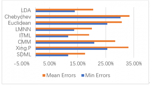
Each DML algorithm was trained by the disturbed Yale face dataset, and then uses a k-nearest neighbors (k-NN) algorithm [21] to classify the test images. The application of each algorithm was repeated ten times and the mean value of the results was taken as the final result. The classification error of each algorithm trained on the disturbed Yale face dataset is displayed in Figure 3.
As shown in Figure 3, the SDML is superior to other seven DML algorithms in most cases. The superiority is attributable to the SDML’s good performance under the serious semantic gap in the test data. Our algorithm can measure the similarity between samples more accurately than the contrastive algorithms.
Next is the comparison of training time. Since Euclidean and Chebychev DML algorithms need no training, the training times of the remaining six DML algorithms were obtained through experiment (Table 1 and Table 2).
The CMM and the LDA algorithms directly decompose data features, eliminating the need of iterative training to obtain an analytical solution. As a result, the two algorithms consumed shorter training times than the other DML algorithms. As shown in Tables 1 and 2, the SDML algorithm consumed less time in training than the ITML and the LMNN. Our algorithm is very sensitive to the dimension of training samples, and its training time increased rapidly with the growth of dimension. Meanwhile, the training time of our algorithm increased slowly with the growing number of training samples.
Figure 3. Image classification errors after training on disturbed Yale face dataset
Table 1. Training time with disturbed Yale face dataset containing different number of training samples
|
Number of training samples |
200 |
250 |
300 |
350 |
400 |
450 |
|
Xing. P |
0.491 |
0.587 |
0.592 |
0.598 |
0.607 |
0.610 |
|
CMM |
0.002 |
0.002 |
0.003 |
0.004 |
0.007 |
0.009 |
|
ITML |
7.128 |
7.219 |
7.287 |
7.307 |
7.318 |
7.482 |
|
LMNN |
9.882 |
9.981 |
10.123 |
12.761 |
14.721 |
16.923 |
|
LDA |
0.872 |
0.896 |
0.908 |
0.918 |
0.932 |
0.971 |
|
SDML |
0.981 |
0.987 |
0.991 |
0.999 |
1.021 |
1.082 |
Table 2. Training time with disturbed Yale face dataset containing training samples of different dimensions
|
Dimensions of training samples |
20 |
40 |
60 |
80 |
100 |
120 |
|
Xing. P |
0.473 |
0.817 |
0.886 |
1.271 |
1.682 |
2.875 |
|
CMM |
0.010 |
0.005 |
0.006 |
0.003 |
0.011 |
0.015 |
|
ITML |
3.826 |
5.821 |
8.725 |
9.921 |
12.341 |
15.821 |
|
LMNN |
5.925 |
7.983 |
8.690 |
9.035 |
15.823 |
18.723 |
|
LDA |
0.736 |
0.756 |
0.842 |
0.982 |
1.254 |
1.862 |
|
SDML |
0.927 |
1.472 |
2.891 |
3.481 |
4.102 |
5.986 |
This paper develops a novel supervised DML algorithm called the SDML, which couples geometric mean and normalized dispersion to balance all inter-class dispersions. Once the similarity distribution of images from different classes is balanced in the metric space, the similarity metric of images will no longer be negatively affected by the semantic gap. In addition, the SDML algorithm uses the MMC to enhance the discrimination ability of the distance metric. The distance between samples from different classes is maximized, promoting the classification accuracy of samples.
Through repeated experiments, the SDML algorithm was proved effective in several aspects. For instance, the algorithm can maintain the consistency between image features and semantic information. The wrong correlation between samples, which is induced by the imbalance of sample distribution, can be avoid by the effective distance metric constructed by our algorithm. Moreover, SDML algorithm can distinguish images from similar classes at a high accuracy.
However, the SDML algorithm is not fast enough to support real-time processing of some computer vision tasks, such as target tracking. This is because the optimization process of our algorithm relies on iterative optimization such as gradient ascent and iterative map. Hence, the future research will focus on creating a faster DML algorithm.
[1] Chan, K.Y., Kwong, C.K., Hu, B.Q. (2012). Market segmentation and ideal point identification for new product design using fuzzy data compression and fuzzy clustering methods. Applied Soft Computing, 12(4): 1371-1378. https://doi.org/10.1016/j.asoc.2011.11.026
[2] Chen, Z., Huang, W., Lv, Z. (2015). Towards a face recognition method based on uncorrelated discriminant sparse preserving projection. Multimedia Tools & Applications, 76(17): 1-15. https://doi.org/10.1007/s11042-015-2882-0
[3] Tai, M., Kudo, M. (2019) A supervised laplacian eigenmap algorithm for visualization of multi-label data: SLE-ML. In: Nyström I., Hernández Heredia Y., Milián Núñez V. (eds) Progress in Pattern Recognition, Image Analysis, Computer Vision, and Applications. CIARP 2019. Lecture Notes in Computer Science, 11896. Springer, Cham. https://doi.org/10.1007/978-3-030-33904-3_49
[4] Li, X.H., Shu, L., Hu, H.L. (2009). Kernel-based nonlinear dimensionality reduction for electrocardiogram recognition. Neural Computing & Applications, 18(8): 1013-1020. https://doi.org/10.1007/s00521-008-0231-1
[5] Gui, J., Sun, Z.N., Jia, W., Hu, R.X., Lei, Y.K., Ji, S.W. (2012). Discriminant sparse neighborhood preserving embedding for face recognition. Pattern Recognition, 45(8): 2884-2893. https://doi.org/10.1016/j.patcog.2012.02.005
[6] Zhang, L., Qiao, L., Chen, S. (2010). Graph-optimized locality preserving projections. Pattern Recognition, 43(6): 1993-2002. https://doi.org/10.1016/j.patcog.2009.12.022
[7] Lu, G.F., Lin, Z., Jin, Z. (2010). Face recognition using discriminant locality preserving projections based on maximum margin criterion. Pattern Recognition, 43(10): 3572-3579. https://doi.org/10.1016/j.patcog.2010.04.007
[8] Sui, Y., Zhang, S., Zhang, L. (2015). Robust visual tracking via sparsity-induced subspace learning. IEEE Transactions on Image Processing A Publication of the IEEE Signal Processing Society, 24(12): 4686-700. https://doi.org/10.1109/TIP.2015.2462076
[9] Qiao, L.S., Chen, S.C., Tan, X.Y. (2010). Sparsity preserving projections with applications to face recognition. Pattern Recognition, 43(1): 331-341. https://doi.org/10.1016/j.patcog.2009.05.005
[10] Hui, K.H., Li, C.L., Zhang, L. (2013). Sparse neighbor representation for classification. Computer Engineering and Design, 33(5): 661-669. https://doi.org/10.1016/j.patrec.2011.11.010
[11] Barazandeh, B., Bastani, K., Rafieisakhaei, M., Kim, S., Kong, Z.Y., Nussbaum, M.A. (2017). Robust sparse representation-based classification using online sensor data for monitoring manual material handling tasks. IEEE Transactions on Automation Science & Engineering, PP(99): 1-12. https://doi.org/10.1109/TASE.2017.2729583
[12] Hayden, D.S., Chien, S., Thompson, D.R., Castaño, R. (2012). Using clustering and metric learning to improve science return of remote sensed imagery. Acm Transactions on Intelligent Systems & Technology, 3(3):1-19. https://doi.org/10.1145/2168752.2168765
[13] Keyhanipour, A.H., Moshiri, B., Piroozmand, M., Oroumchian, F., Moeini, A. (2016). Learning to rank with click-through features in a reinforcement learning framework. International Journal of Web Information Systems, 12(4): 448-476. https://doi.org/10.1108/IJWIS-12-2015-0046
[14] Li, X., Bai, Y.Q. (2017). Convergence analysis of an intrinsic steepest descent method on semi-supervised metric learning. Operations Research Transactions, 21(3): 1-13. https://doi.org/10.15960/j.cnki.issn.1007-6093.2017.03.001
[15] Liang, J., Ren, L.Y., Ju, H.J., Qu, E.S., Wang, Y.L. (2014). Visibility enhancement of hazy images based on a universal polarimetric imaging method. Journal of Applied Physics, 116(17): 173107. https://doi.org/10.1063/1.4901244
[16] Wang, M., Hua, X.S., Tang, J.H., Hong, R.C. (2009). Beyond distance measurement: constructing neighborhood similarity for video annotation. IEEE Transactions on Multimedia, 11(3): 465-476. https://doi.org/10.1109/TMM.2009.2012919
[17] Hu, Q.H., Zhu, P.F., Yang, Y.B., Yu, D. (2011). Large-margin nearest neighbor classifiers via sample weight learning. Neurocomputing, 74(4): 656-660. https://doi.org/10.1016/j.neucom.2010.09.006
[18] Johnson, D.M., Xiong, C.M., Corso, J.J. (2014). Semi-supervised nonlinear distance metric learning via forests of max-margin cluster hierarchies. IEEE Transactions on Knowledge & Data Engineering, 28(4): 1035-1046. https://doi.org/10.1109/TKDE.2015.2507130
[19] Wang, J., Wang, Z., Liang, C., Gao, C.X., Sang, N. (2018). Equidistance constrained metric learning for person re-identification. Pattern Recognition, 74: 38-51. https://doi.org/10.1016/j.patcog.2017.09.014
[20] Wang, H.S., Li, G.D., Tsai C.L. (2007). Regression coefficient and autoregressive order shrinkage and selection via the lasso. Journal of the Royal Statistical Society, 69(1): 63-78. https://doi.org/10.1111/j.1467-9868.2007.00577.x
[21] Rasheed, S., Stashuk, D., Kamel, M. (2008). A software package for interactive motor unit potential classification using fuzzy k-NN classifier. Computer Methods and Programs in Biomedicine, 89(1): 56-71. https://doi.org/10.1016/j.cmpb.2007.10.006VVVV