Xun Li | Chuan Lin | Xinpeng Xu*
© 2019 IIETA. This article is published by IIETA and is licensed under the CC BY 4.0 license (http://creativecommons.org/licenses/by/4.0/).
OPEN ACCESS
Target tracking is the key function of intelligent production monitoring systems in manufacturing enterprises. In many monitoring systems, however, the fields of view (FOVs) of multiple cameras only partially overlap each other, leaving many blind zones that affect the target tracking effect. To solve the problem, this paper explores the spatial correlation probability of appearance features, and discusses about the brightness transfer function (BTF) between different FOVs. Next, the effects of appearance matching were improved, the target position was reconstructed in world coordinate system, and the spatial features of the target was extracted. On this basis, the author established a target tracking and matching appearance model with spatial information. Finally, the effectiveness of the model was fully verified through a simulation on the multi-camera production monitoring system of a factory.
target tracking, appearance features, spatial information, multi-plane projection
Production monitoring systems have been widely adopted in today’s enterprises [1]. These systems should realize intelligent monitoring of the production line, and achieve comparable performance as manual monitoring. Modern production enterprises often operate several production lines at the same time. Therefore, multiple distributed cameras should be arranged in the intelligent production monitoring system to track the targets on each production line, analyze the target behavior, and detect abnormalities in time.
The multi-camera monitoring system boasts a larger monitoring range and a wider view angle than single-camera monitoring system. As a result, the information of moving targets can be captured comprehensively, even in the presence of occlusions. However, the introduction of multiple cameras has brought a new problem: the fields of view (FOVs) of some cameras only partially overlap each other, leaving blind zones between them. If a target passes through or remains in a blind zone, the monitoring system will lose the target. When the target reenters the monitoring range, the system must associate it with the previously detected target to realize continuous tracking. For cameras with blind zones, the difficulty of continuous tracking is further increased by the fact that the same target appears differently in these cameras. The different appearances come from the varied FOVs and illuminations between the cameras.
To solve the problem, this paper fully explores the target matching and tracking of multi-camera production monitoring systems with blind zones. Drawing on the existing technologies, the trajectory of the target moving across the FOVs of multiple cameras was reconstructed, and the motion features of the target were extracted. The reconstruction and feature extraction were carried out based on spatial information. In this way, the multiple cameras can realize smooth handover of the target, and associate the reappearing target with the previously detected target, that is, achieve continuous tracking of the target in the presence of blind zones. The research results shed theoretical lights on intelligent production monitoring systems.
The target tracking by multiple cameras [2] is an interdisciplinary issue, involving technologies like computer vision and pattern recognition. In the presence of blind zones, target appearance differs greatly from camera to camera, making the single-camera tacking algorithm inapplicable. To solve the target tracking problem of multiple cameras with blind zones, the traditional approaches mainly include appearance model [3], spatiotemporal correlation algorithm, and data fusion.
The appearance model usually extracts correlation features like color and texture from the regions of interest (ROIs) of images or video frames on different targets, and then evaluates the similarity between these targets. Ordonez-Etxeberria et al. [4] calculated the main color spectrum of each target based on the distance of color space, and compared the distance between different targets. Nonetheless, the direct use of color and color-related features lacks spatial information, making the model matching less effective. Yilmaz et al. [5] divided the image into three parts by aspect ratio, and realized histogram matching in two layers: the first layer is the entire target, and the second is the three parts of the target. Nam et al. [6] meshed the target into multiple grids, and matched the features between the grids. Lo et al. [7] established a complex three-dimensional (3D) model, sampled images with the model and camera calibration parameters, and reconstructed the 3D model of the target to complete the matching process.
Considering the difference of multiple cameras in target appearance, it is very important to set up a robust model to convert the colors between different cameras. The color transfer model between cameras should be corrected to improve the matching accuracy. Wang et al. [8] proposed a brightness transfer algorithm through sample training. Based on the multiple targets in the sample set, the algorithm learns the subspace of the brightness transfer function (BTF) through probabilistic principal component analysis (PCA), thus reducing the brightness difference between targets. Sun et al. [9] combined mean brightness transfer function (MBTF) with cumulative brightness transfer function (CBTF), and achieved good color conversion effects through BTF subspace learning.
The spatiotemporal correlation algorithm estimates the probability of correlation between targets passing through the blind zones, using the information on position, time, speed and moving direction. The blind zones between multiple cameras are either long-distance ones or short-distance ones. The two types of blind zones should be processed with different algorithms. The correlation algorithm of short-distance blind zones [10] is essentially an extension of the single-camera tracking algorithm. Since the blind zones are very small, the target can be located by predicting the target motion with the classical particle filter and Kalman filter. The correlation algorithm of long-distance blind zones [11] is mainly based on statistical learning algorithm of camera correlation. During the training process, the algorithm estimates the transfer probability between cameras to determine the probability of matching.
The appearance model or spatiotemporal correlation algorithm alone cannot fully solve the continuous tracking of target in the presence of blind zones. In many cases, multiple targets may have high similarity in some feature correlations. These features should be obtained from multiple models and fused together. Besides, it should be noted that a target can only be associated with another target, i.e. the relationship is unique. A common method for data fusion is the maximum probability distribution algorithm, which is the basis for probability model. Baltieri et al. [12] used the matching algorithm of appearance model to identify the similarity between targets, computed the correlation probability based on the spatiotemporal features of targets (i.e. position, time and speed), and determined the similarity by multiplying the similarity and the probability. Wang et al. [13] developed a framework of target correlation based on fuzzy logic theory, computed the set of maximum probabilities of target correlations, and thus derived the global correlation between multiple targets.
Currently, target trajectory in space is usually reconstructed according to the information extracted from video sequence. On this basis, the direction of the trajectory can be obtained, and the correlation between camera FOVs can be matched. The trajectory contains spatiotemporal features of the correlation. In addition to these features, the appearance features like color, texture, contour and gait can also be used to track target in blind zones.
In the intelligent production monitoring system, the target is an image sequence containing the monitoring information of camera FOVs, rather than a static image. This type of information cannot be fully utilized by traditional matching algorithms, such as the PCA based on spatial distribution entropy and the BTF subspace algorithm.
To overcome the above defects, this paper firstly estimates the height of the target by multiplane projection. The height was selected because it is a relatively stable appearance feature. For the same target, the height will not change obviously through the movement, ensuring the matching accuracy between the reappearing and previous targets. Next, the BTF between cameras was trained to compensate for the color deviation of the target appearance in different FOVs. Based on the spatial information of the target (i.e. height, moving direction and position), the relationship between the color space and image position was established. After that, the position of the reconstructed color space was used to weight different color spaces, and to increase the spatial distribution information of color features. In this way, multiple images were fused to enhance the matching accuracy.
3.1 Height estimation through multiplane projection
Firstly, a world coordinate system was set up with the x- and y- axis on the horizontal plane (z=0) and the z-axis perpendicular to the horizontal plane. The target was originally placed on the plane $P_{0}$. The plane with a distance h above $P_{0}$ is denoted as plane $P_{h}$. Using the pinhole model and calibration parameters of cameras, the foreground pixels of the target were projected onto different planes, including $P_{0}$ and a series of planes $P_{h}$. The mapping rule between different planes satisfies the geometric relationship.
Let $\left(x_{a}, y_{a}\right)$ be the camera position on the horizontal plane and $h_{a}$ be the height of the camera. For point O on plane $P_{0}$, the coordinates of its projection point P on plane $P_{h}$ and those of its projection point Q on the horizontal plane satisfy the following relationships:
$x_{p}=x_{q}-\left(x_{q}-x_{a}\right) z_{p} / h_{a}$
$y_{p}=y_{q}-\left(y_{q}-y_{a}\right) z_{p} / h_{a}$ (1)
The vertical axis w of the target is perpendicular to $P_{0}$. If looking down vertically to $P_{0}$, the target projection on the horizontal plane must extend away from the camera, and that on $P_{h}$ must fall on the other side of w. Then, the plane at the target height $P_{h}$ ends at w, the $P_{0}$ begins at w, and the two projections intersect at $\left(x_{v}, y_{v}\right)$.
Hence, the coordinates $p(x, y)$ of the target projection on the horizontal plane were obtained by the trajectory reconstruction algorithm based on multi-feature points. Then, the total distance between the projection and the target was acquired by multiplane projection, and the minimum height of the total distance was taken as the target height.
Let $\varphi$ be the set of foreground pixels of the target, and $\mathrm{X}_{i}^{h}$ be position of foreground pixel i in $\varphi$, with h being the height that the pixel is projected to in the world coordinate system. Then, $\mathrm{X}_{i}^{h}$ was projected to the horizontal plane to obtain the position $x_{i}$ of the common FOV. Let $D\left(x_{i}, p\right)$ be the Euclidean distance from $x_{i}$ to the target position p. Thus, the total projection distance $L_{h}$ of all foreground pixels can be expressed as:
$L_{h}=\sum_{i \in \varphi}\left(x_{i}^{h}, p\right)$ (2)
In fact, there is no need to find the global optimal solution of $L_{h}$, due to the limited calibration accuracy and the possible errors induced by the extraction of foreground pixels and the reconstruction error of target position.
In actual computation, the minimum interval of projection plane is 0.1 cm and $L_{h}$ is a convex function of h. Thus, the minimum projection height h was calculated every other 1cm. Twenty planes, h1-10~ h1+10, were projected by the interval of 0.1cm to obtain the total projection distance of foreground pixels. Then, the projection height corresponding to the minimum total value was adopted as the target height.
According to the law of target motion, the center of gravity of the moving target tends to rise and fall periodically. Being a correlation feature of the target, the height can be used to screen out targets with marked differences. But this strategy faces two major defects. For one thing, the target height may vary slightly during the motion, causing changes in the number of pixels on the image plane. The farther the target moves, the smaller its contour on the image, and the greater the estimation error. For another, the target height estimated in different FOVs may have systematic error, owing to calibration error and other reasons. The following strategy was adopted to solve the defects.
First, the target height in each frame was estimated by multiplane projection. Next, the mean height H was obtained by averaging the estimated results of multiple frames. Meanwhile, the height interval dH was determined based on the FOVs of different cameras. The estimated results that fall out of the dH were removed, leaving only those within this interval. After that, the systematic error in target height estimation was defined as a linear function:
$H_{j, a}=f_{i, j}^{H}\left(H_{i, a}\right)=\alpha H_{i, a}+\varepsilon$ (3)
where, $H_{i, a}$ and $H_{j, a}$ are the heights of target a estimated in the FOVs of cameras $C_{i}$ and $C_{j}$, respectively; $\alpha$ and $\varepsilon$ are height transfer parameters between cameras that can be estimated through linear fitting of sample data. The similarity between $H_{i, a}$ and $H_{i, a}$ can be obtained as:
$P_{H}\left(O_{i, a}, O_{j, b}\right)=\exp \left(-\left(O_{i, a}(H)-f_{i, j}^{H} * O_{j, b}(H)\right)^{2} / \sigma_{H}^{2}\right.$ (4)
3.2 HSV histogram matching based on spatial information
For simplicity, the traditional appearance model algorithms usually extract color features from the target area for comparison. To match color features, the color space must be selected rationally, the color features quantized into vectors, and a similarity (distance) criterion defined to measure color similarity between images. Unlike other visual features, color features are not heavily dependent on the size, direction or perspective of the image, and highly invariant to rotations.
Despite the high rotation-invariance, the color features are easy to lose spatial information, which is inconducive to feature matching. For example, it is impossible to distinguish between a black-and-white target and a white-and-black target by the color histogram features extracted from the color space. In view of this, spatial information is added to color features in most emerging matching algorithms of color-based appearance model.
In the intelligent production monitoring system, the target is not an isolated image, but an image sequence. To achieve effective matching, the color-based appearance model must fuse multi-frame images from different angles. Traditionally, the multiple images are processed by the weighted average method. However, the weighted features will be close to the original ones, if the pixel features are different between the front and back planes of a target. In this case, the fused target will be matched with the wrong target. To solve the problem, this paper proposes the HSV histogram matching algorithm based on spatial information. The algorithm firstly trains the BTF between cameras, and uses the trained BTF to compensate for the color deviation of target appearances in different FOVs. After that, the targets in different FOVs were matched.
In the multi-camera monitoring system with blind zones, each camera has a unique illumination conditions that affects the color features of target. The target is bright under strong illumination, and dark under weak illumination. The varied brightness makes it more difficult to predict the impacts of shadows and occlusion. The color difference of the same target is further amplified, because different cameras often use different photosensitive devices. There are two ways to eliminate this color difference: finding the features insensitive to illumination, and creating the BTF [14] between cameras. The latter strategy is adopted here.
The reflection coefficient $R_{s}(o, t)$ of target o under the FOV s at time t can be expressed as:
$R_{S}(o, t)=M(o) G_{S}(o, t)$ (5)
where, $M(o)$ is the reflection coefficient of the target material; $G_{S}(o, t)$ is the influence of camera geometry and target time variation. It is assumed that all points on the target image satisfy $G_{S}(o, t)=G_{S}(q, t)=G_{S}(t)$, i.e. the target has a flat surface. Then, the time-variation of camera’s internal parameters can be defined as:
$Y_{S}(t)=\frac{\pi}{4}\left(\frac{d_{S}(t)}{h_{S}(t)}\right)^{2} \cos ^{4} \alpha_{S}(o, t)=\frac{\pi}{4}\left(\frac{d_{S}(t)}{h_{S}(t)}\right)^{2} C$ (6)
where, $h_{s}(t)$ is focal length; $d_{s}(t)$ is lens size; $\alpha_{s}(o, t)$ is the angle between the optical axis and the line between optical center and p.
Then, the brightness $B_{S}(o, t)$ of point o on the target image can be expressed as:
$B_{S}(o, t)=g_{s}\left(E_{S}(o, t) X_{S}(t)\right)=g_{s}\left(M(o) G_{S}(t) Y_{S}(t) X_{S}(t)\right)$ (7)
where, $X_{s}(t)$ is exposure time, and $g_{s}()$ is the radiation response function of the camera.
For the same target, the material is the same under different cameras. Hence, $M(o)$ can be derived from formula (7) as:
$M(o)=\frac{g_{s}^{-1}\left(B_{S}\left(o, t_{s}\right)\right)}{G_{S}\left(t_{S}\right) Y_{S}\left(t_{S}\right) X_{S}\left(t_{S}\right)}=\frac{g_{u}^{-1}\left(B_{u}\left(o, t_{u}\right)\right)}{G_{u}\left(t_{u}\right) Y_{u}\left(t_{u}\right) X_{u}\left(t_{u}\right)}$ (8)
Then, we have:
$\begin{aligned} B_{u}\left(o, t_{u}\right)=& g_{u}\left(\frac{G_{u}\left(t_{u}\right) Y_{u}\left(t_{u}\right) X_{u}\left(t_{u}\right)}{G_{S}\left(t_{S}\right) Y_{S}\left(t_{S}\right) X_{S}\left(t_{S}\right)} g_{S}^{-1}\left(B_{S}\left(o, t_{S}\right)\right)\right)=\\ & g_{u}\left(w\left(t_{S}, t_{u}\right) g_{S}^{-1}\left(B_{S}\left(o, t_{S}\right)\right)\right.\end{aligned}$ (9)
Formula (9) shows, for any point on the target image, the BTF between different frames are obviously different. The parameters p, $t_{s}$ and $t_{u}$ are negligible. Let $f_{s u}$ be the BTF of camera $C_{s}$ to camera $C_{u}$. Then, we have:
$B_{u}=g_{u}\left(w g_{s}^{-1}\left(B_{s}\right)=f_{s u}\left(B_{s}\right)\right.$ (10)
In BFT research, the normalized cumulative histograms, i.e., the integration of the normalized histograms on the grayscale, are often adopted. Let $H_{s}$ and $H_{u}$ be the normalized cumulative histograms of targets $O_{s}$ and $O_{u}$, respectively. Then, $H_{S}\left(B_{S}\right)=H_{u}\left(B_{u}\right)=H_{u}\left(f_{s u}\left(B_{u}\right)\right)$. Then, the following equation can be derived:
$f_{s u}\left(B_{s}\right)=H_{u}^{-1}\left(H_{s}\left(B_{s}\right)\right)$ (11)
To set up the color histogram, the color space was divided into several intervals according to the resolution or length of the histogram. Each interval corresponds to a bin of the histogram. Then, the target image area was traversed, and the pixels falling into the corresponding color space were counted to obtain the color distribution. Let $H(k)$ be the vector of the color histogram. Then, the color histogram conversion can be defined as:
$H_{k}=\frac{n_{k}}{N}(k=0,1, \ldots, L-1)$ (12)
where, k is a dimension of the vector; L is the number of bins in the color histogram; $n_{k}$ is the number of pixels in the color space corresponding to k in the target image area; N is the total number of pixels in the image.
3.3 Appearance model based on spatial information
In this section, the target height is estimated by multiplane projection. Then, the color-based model with spatial information was established for each target based on the target heights. Moreover, the relationship between color space and target position was reconstructed, and used to determine the spatial information of the color space.
To begin with, the author set up a cylinder with the origin as the center, the height of $h_{0}$=1 and the radius of *$h_{0}$. Then, the cylinder surface was divided into M layers, and each layer was further meshed into N grids. From the intersection of the cylinder and the x-axis, the grids were numbered from 1 to N in counterclockwise order.
Next, the direction vector of the first block $\overrightarrow{f_{0}}=(1,0,0)$ was taken as the direction of the model, and the central point of the target was viewed as the position of each block. Let $\overrightarrow{n_{l}}(i=1,2, \ldots, M * N)$ be the direction vector perpendicular to the cylinder. Then, the grids $p_{S}(x, y, z)(i=1,2, \ldots, M * N)$ of the $M * N$ points of the model and their direction vectors $\overrightarrow{n_{l}}$, and the positive direction vector $\overrightarrow{f_{0}}$ of the model were obtained.
Let $p(x, y, z)$, height and orientA be the position, height and direction of target A in world coordinate system, respectively. If z=0, then the target is on the horizontal plane. The position of each grid was updated by increasing the height. Then, the position of each point $(s=1,2, \dots, M * N)$ can be updated by:
$p_{s}(x, y, z)=$height$* p_{s}(x, y, z)$ (13)
On the other hand, it is assumed that $\overrightarrow{f_{0}}$ rotates to orient $_{A}$ by a counterclockwise angle of $\theta$ (both vectors are parallel to the horizontal plane). Then, all the grids $p_{s}(x, y, z)$ and the corresponding normal vectors were rotated by $\theta$ around the z-axis, making the target direction the positive direction of the model.
Finally, all updated and rotated points $p_{s}(x, y, z)$ were translated to $p(x, y, z)$, such that the center points moved (0,0,0) to the final positions $p(x, y, z)$. These grids were projected back to the image plane, creating new gird $c_{s}(x, y)(s=1,2, \dots, M * N)$. In this way, the author determined the correspondence between color space and target position. The cylindrical model and projected grids are shown in Figure 1.
Figure 1. The cylindrical model
In the cylindrical model, the grids on the back were covered by those facing the camera. The occlusion was not reflected after the grids were projected back to the image plane. To represent the occlusion, the normal vectors p of the image plane were calculated based on camera’s calibration parameters, and subjected to dot multiplication with the direction vectors of the dot matrix: $\theta=\vec{n} \cdot \vec{p}$. The $\theta$ value was negative for the grids on the back and positive for those on the front. The greater the $\theta$ value, the more visible the corresponding grid.
For a target entering the FOV, an instance $\Gamma$ was established for it by zooming, rotating and translating the original model: $\Gamma=\left\{\text { position, height, orient },\left\{V^{M * N}\right\}\right.$, where position, height and orient are the height, position and direction of the target, respectively; $\left\{V^{M * N}\right\}$ is the feature set of $M * N$ grid centers. Each V is a combination of three parameters:
(1) $\overrightarrow{n_{l}}$: This parameter is the normalized cylindrical normal vector of grid center.
(2) $H_{i}$: This parameter is the HSV histogram of grid i on the image plane. Let $c_{s}(x, y)$ be the projection of the center of grid i on the image plane. Then, the $H_{i}$ of the foreground pixels in the image area (size: patch $_{N} *$ patch $_{-} N$) centering on $c_{s}(x, y)$ was calculated. After that, H was quantified into 8 units, while S and V were quantified into 4 units. Then, the three histograms were merged into a large histogram, which was then normalized into histogram $H_{i}$. Note that patch_ $N$ was selected according to the height of $i m a g_{-} H$ of the target foreground pixel and the number of layers of the selected points. The patch_ $N$ value should not be excessively large or small. Here, it is set to $N=a l f * i m a g_{-} H / M$.
(3) reliable $_{i}$: This parameter measures the reliability of the grid area. It was obtained through dot multiplication of the normal vector of grid center $\overrightarrow{\eta_{l}}$ and that of the image plane $\vec{p}$.
If the image area (size: patch_n * patch_N) is partially invisible, then the invisible part is not covered in the $H_{i}$ calculation. If the entire area is invisible, then the image area is invalid and its $reliable_{i}$ is set to -2.
3.4 Target tracking and matching by the appearance model with spatial information
This subsection explains how to apply the established appearance model in target tracking and matching of multi-camera monitoring system with blind zones.
The first step is to initialize the system configuration, including calibration, installation, time sync, and alignment of cameras. Then, the FOV boundary of each camera was marked with points, and mapped to a horizontal plane. In addition, the BTF $f_{s u}$ between cameras $C_{s}$ and $C_{u}$ was trained.
Taking camera $C_{i}$ as an example, each target $O_{i, a}$ entering the camera’s FOV was tracked continuously by the single-camera tracking algorithm. The foreground pixels of the target were extracted. After a period (time window) Twin, the target trajectory $O_{i, a}(\operatorname{tr} a)$ was reconstructed in the horizontal plane by the trajectory reconstruction algorithm, and the trajectory features were extracted. If the target is completely visible (i.e. the target is in the lens and the reconstructed position falls in the FOV), the target height $H_{i, a}^{t}$ can be obtained by multi-plane projection.
It is assumed that camera $C_{j}$ has a set of N sets $O_{j}\left\{O_{j, 1}, O_{j, 2}, \ldots, O_{j, N}\right\}$ and camera $C_{I}$ has a set of M targets $O_{i}\left\{O_{i, 1}, O_{i, 2}, \ldots, O_{i, N}\right\}$ before time t. The targets have been detected (i.e. the targets that have entered and left the FOV) and those being detected under a single camera were allocated to the observation set. To track each target, all the targets must be matched to reveal the relationship between targets and time sequence.
Let $P_{s t}\left(O_{i, a}, O_{j, b}\right)$ be the correlation probability between $O_{i, a}$ and $O_{j, b}$, $P_{H}\left(O_{i, a}, O_{j, b}\right)$ be the height similarity between the two targets, and $P_{H S V}\left(O_{i, a}, O_{j, b}\right)$ be the similarity of HSV histogram based on spatial information. Then, the final similarity between the two targets can be determined as:
$P_{a p p}\left(O_{i, a}, O_{j, b}\right)=P_{H}\left(O_{i, a}, O_{j, b}\right) * P_{H S V}\left(O_{i, a}, O_{j, b}\right)$ (14)
Ultimately, the correlation probability between $O_{i, a}$ and $O_{j, b}$ is the weighted sum of the spatiotemporal correlation probability and the external model correlation probability.
$P\left(O_{i, a}, O_{j, b}\right)=$$P_{H}\left(O_{i, a}, O_{j, b}\right) * P_{H S V}\left(O_{i, a}, O_{j, b}\right) * P_{s t}\left(O_{i, a}, O_{j, b}\right)$ (15)
Next, it is assumed that $\Sigma$ is the solution space of the multi-camera tracking problem, and $K=\left\{K_{i, a}^{j, b}, K_{p, c}^{r, e} \ldots\right\}$ is one of the associated subsets of the problem. For any $K_{i, a}^{j, b} \in K$, there exists $\phi_{K_{i, a}^{j, b}}=1$. Since each target can only be associated with one previous or subsequent target, the subset K can be described as $\phi_{K}=$ true for any $\left\{K_{i, a}^{j, b}, K_{p, c}^{r, e}\right\} \in K,(i, a) \neq(p, c) \wedge(j, b) \neq(r, e)$, which is a feasible solution in the solution space. Therefore, the tracking problem is to find the maximum likelihood probability in all feasible solutions in the solution space $\Sigma$:
$K^{\prime}=\operatorname{argmax}_{K \in \Sigma} \prod P\left(O | \phi_{K}=\text { true }\right)$ (16)
If the correlation probability between any two targets is independent to that of any other two targets, then the above formula can be rewritten as:
$K^{\prime}=\operatorname{argmax}_{K \in \Sigma} \prod_{K_{i, a}^{j, b} \in K} P\left(O_{i, a}, O_{j, b} | \phi_{K_{i, a}^{j, b}}=\operatorname{tr} u e\right)$ (17)
Taking logarithms on both sides of formula (17), and the problem is transformed into solving the maximum of the summation equation below:
$K=\operatorname{argmax}_{K \in \Sigma} \sum_{K_{i, a}^{j, b} \in K} \log P\left(O_{i, a}, O_{j, b} | \phi_{K_{i, a}^{j, b}}=\operatorname{tr} u e\right)$ (18)
The above algorithm assumes that all observation sets are known and available. To make it suitable for real time series, a fixed interval sliding time window should be added to the algorithm to calculate the correlations between all targets in the window. If the time window is too long, the matching will have a long delay; if the time window is too short, the matching results will contain a high error. Hence, the window size should be defined to cover the matching time of all the cameras.
To verify the effectiveness of our model and algorithm, a test sequence was collected from a production monitoring system with four cameras (frame rate: 20fps) in a factory. The four cameras have no overlap between the FOVs. Each camera has been calibrated by Tsai’s method and aligned to a unified world coordinate system.
Based on the camera’s calibration parameters, the FOVs of the four cameras were projected onto the horizontal plane (z=0). As shown in Figure 2, there were only a few very small overlaps between the four FOV projections.
Figure 2. Projection of the FOVs in the horizontal plane (z=0)
Figure 3 shows the reconstructed trajectory of a target on the horizontal plane. Only the upper half of the target appeared in the FOV of Camera 3. The trajectories of the target were reconstructed by the trajectory reconstruction algorithm in the blind zones, and linked up with that in each of the other three FOVs. The trajectories were closed to each other at the joints, rather than identical, due to the calibration error (the feature points extracted from different cameras were not the same physical point). As shown in Figure 3, the reconstructed trajectory in the FOV of Camera 3 was different from the other trajectories. The mean distance of the overlap point of the camera was 0.12 m. For the parts produced in the workshop, the space occupies about 0.6*0.8 m. This distance can be used to correlate the targets of different cameras.
Figure 3. The reconstructed trajectory of a target on the horizontal plane (z=0)
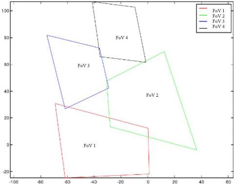
Next, the FOVs of Cameras 1 and 4, which are not overlapped, were used to correlate the target trajectories. The projections of the two FOVs are shown in Figure 4.
Figure 4. Projections of two nonoverlapped FOVs
The correlation probability between the trajectories in the two FOVs was computed in the above two scenes, with the time window of 30s. There were 5 trajectories in the FOVs of Camera 4 and 9 in that of Camera 1. The results are listed in Table 1.
From which we can get that our model successfully reconstructed the position of the moving target on the horizontal plane based on partially visible image sequences, and achieved the tracking of the target moving in the production line of a factory.
Table 1. The correlation probability for Cameras 1 and 4
|
|
Trajectories of Camera 1 |
1 |
2 |
3 |
4 |
5 |
|
Trajectories of Camera 4 |
|
|
|
|
|
|
|
1 |
|
- |
- |
15.5% |
- |
5.5% |
|
2 |
|
- |
- |
- |
- |
- |
|
3 |
|
- |
92.5% |
3.2% |
- |
0.2% |
|
4 |
|
- |
- |
- |
- |
- |
|
5 |
|
- |
- |
70.8% |
- |
1.8% |
|
6 |
|
- |
- |
- |
- |
- |
|
7 |
|
- |
- |
- |
- |
26.6% |
|
8 |
|
- |
- |
- |
- |
62.5% |
|
9 |
|
- |
- |
- |
- |
- |
In the intelligent production monitoring system, there are often nonoverlapping areas between the FOVs of different cameras. These blind zones make it difficult to track targets passing across multiple cameras. To solve the problem, this paper probes deep into the BTF between different FOVs, and relied on the BTF to improve the effects of appearance matching. Next, the target position was reconstructed in world coordinate system and the spatial features of the target was extracted. Finally, a target tracking and matching appearance model was established based on the 3D spatial information, and proved capable of accurate matching between targets in the image sequences captured by multiple cameras with blind zones.
The authors acknowledge funding from the key project of Chongqing Municipal Education Commission Humanities and Social Sciences Base Project (18SKJD036), Science and Technology Project of Chongqing Education Commission (KJQN201800904), Ministry of education of Humanities and Social Science Project of China (18YJC630087), Sichuan International Studies University Scientific Research Project (sisu201407) and Sichuan International Studies University Non-Common Language Research Team Project, as well as the contributions from all partners of the mentioned projects. Besides, Xu Xinpeng is the corresponding author and can be contacted at: xinpengxu@cqu.edu.cn.
[1] Liu, D.C., Zheng, Y., Dai, L., Cheng, L.H., Zheng, L. (2005). Research on the monitor effective information based remote video processing technology. Computer Integrated Manufacturing System, 11(3): 411-415. http://dx.doi.org/10.3969/j.issn.1006-5911.2005.03.020
[2] Qin, Y., Ma, H., Cheng, L., Li, Y., Zhou, X.Q. (2016). Cardinality balanced multitarget multi-Bernoulli filter for multipath multitarget tracking in over-the-horizon radar. Iet Radar Sonar & Navigation, 10(3): 535-545. http://dx.doi.org/10.1049/iet-rsn.2015.0284
[3] Kang, S.B., Jones, M. (2002). Appearance-based structure from motion using linear classes of 3-d models. International Journal of Computer Vision, 49(1): 5-22. http://dx.doi.org/10.1023/a:1019849812326
[4] Ordonez-Etxeberria, I., Hueso, R., Sánchez-Lavega, A., Pérez-Hoyos, S. (2016). Spatial distribution of jovian clouds, hazes and colors from Cassini ISS multi-spectral images. Icarus, 267: 34-50. http://dx.doi.org/10.1016/j.icarus.2015.12.008
[5] Yilmaz, A., Li, X., Shah, M. (2004). Contour-based object tracking with occlusion handling in video acquired using mobile cameras. IEEE Transactions on Pattern Analysis & Machine Intelligence, 26(11): 1531-1536. http://dx.doi.org/10.1109/TPAMI.2004.96
[6] Nam, Y., Rho, S., Park, J.H. (2013). Inference topology of distributed camera networks with multiple cameras. Multimedia Tools & Applications, 67(1): 289-309. http://dx.doi.org/10.1007/s11042-012-0997-0
[7] Lo, K.H., Chuang, J.H. (2013). Vanishing point-based line sampling for real-time people localization. IEEE Transactions on Circuits and Systems for Video Technology, 23(7): 1209-1223. http://dx.doi.org/10.1109/TCSVT.2013.2242592
[8] Wang, S.D., Zhou, D.C., Wang, J. (2012). A moving object detection algorithm based on learning vector quantization. Opto-Electronic Engineering, 39(9): 42-48. http://dx.doi.org/10.3969/j.issn.1003-501X.2012.09.008
[9] Sun, G.X., Bin, S. (2017). Router-level internet topology evolution model based on multi-subnet composited complex network model. Journal of Internet Technology, 18(6): 1275-1283. http://dx.doi.org/10.6138/JIT.2017.18.6.20140617
[10] Qiao, B., Li, Z.C., Hu, P. (2011). Object tracking algorithm based on camshift with dual ROI and velocity information fusion. Information & Control, 40(3): 283-288. http://dx.doi.org/10.1090/S0002-9939-2011-10775-5
[11] Chen, H.T., Tsai, W.J., Lee, S.Y., Yu, J.Y. (2012). Ball tracking and 3D trajectory approximation with applications to tactics analysis from single-camera volleyball sequences. Multimedia Tools & Applications, 60(3): 641-667. http://dx.doi.org/10.1007/s11042-011-0833-y
[12] Baltieri, D., Vezzani, R., Cucchiara, R. (2015). Mapping appearance descriptors on 3D body models for people re-identification. International Journal of Computer Vision, 111(3): 345-364. http://dx.doi.org/10.1007/s11263-014-0747-z
[13] Wang, H.Y., Wang, X., Zheng, J., Deller, J.R., Peng, H.Y., Zhu, L.P., Chen, W.J., Li, X.L., Liu, R.J., Bao, H.J. (2014). Video object matching across multiple non-overlapping camera views based on multi-feature fusion and incremental learning. Pattern Recognition, 47(12): 3841-3851. http://dx.doi.org/10.1016/j.patcog.2014.06.019
[14] Bhandari, A.K., Kumar, A., Singh, G.K., Soni, V. (2016). Dark satellite image enhancement using knee transfer function and gamma correction based on DWT–SVD. Multidimensional Systems and Signal Processing, 27(2): 453-476. http://dx.doi.org/10.1007/s11045-014-0310-7