Kaushal Kumar| Ritesh Kumar Mishra*
© 2019 IIETA. This article is published by IIETA and is licensed under the CC BY 4.0 license (http://creativecommons.org/licenses/by/4.0/).
OPEN ACCESS
Pedestrian detection is a fundamental problem in various computer vision applications and is addressed by complex solutions involving complex feature extractor and classification techniques. In this paper, feature selector is used along with Histogram of Significant Gradients (HSG) descriptor and linear SVM classifier to enhance the detection accuracy and reduce the processing time. A feature selector organizes the extracted features in decreasing order of their significance. A comparative study has been done employing different classifiers and feature selectors and a system is proposed with better detection capability. The proposed scheme is found to have a 50 % reduction in feature size, 67 % reduction in processing time and 3.93 % improvement in accuracy.
classifier, feature selection, HOG, HSG, pedestrian detection, SVM
Robust detection of pedestrian with complex background is a challenging task in computer vision. It helps in a number of applications including smart vehicle, smart surveillance system and human computer interaction. The challenge in pedestrian detection is that the algorithm should provide accurate detection under different illumination conditions. Moreover, due to various poses and variation in clothing that human exhibit makes it a difficult problem in computer vision. For its real time implementation, the algorithm should provide accurate solution in short processing time. All these reasons make pedestrian detection an active area of research. Feature extraction along with classifier is the most common approach followed in pedestrian detection.
Histogram of Oriented Gradients (HOG) in association with linear Support Vector Machine (SVM) classifier is regarded as a better candidate than other single features proposed for detecting pedestrian [1-2]. Bilal et al. [3] proposed a modified version of HOG termed as HSG which has less algorithmic complexity than HOG. In this paper, we have further improved the detection capability of HSG by appending feature selection block. Addition of feature selector will also reduce processing time and results in a robust feature selector. The framework for detecting pedestrian used in this paper is shown in Figure 1.
(a)
(b)
Figure 1. Block diagram of pedestrian detection framework: (a) Training phase (b) Testing phase
It is found that HSG descriptor with linear SVM classifier and mRMR feature selector provides better performance than the approach used without feature selector. The rest of the paper is categorized as follows: Section 2 provides a brief background on research work done in pedestrian detection. Section 3 describes the preliminary work required in this paper. Section 4 provides an outlook into the proposed approach. Section 5 compares the result of the proposed approach with existing method. Section 6 concludes the work focusing important findings.
Now a days, a significant attention has been brought by the computer vision researchers to solve the problem of pedestrian detection in images and videos. Many studies are going on how to effectively extract the pedestrian features. SIFT [4-5], SURF [6], LBP [7-9], HOG[10], EOH [11] and SC [12] are some of the commonly used techniques of feature extraction. Among all such techniques, HOG is found to outperform others in detecting pedestrian. Dalal and Triggs proposed HOG for human detection [10]. HOG is a shape descriptor and remains unaffected by illumination and rotation transformation. Lowe D G et al. initiated Scale Invariant Feature Transform (SIFT) identify key points based on the difference of gaussian (DoG) [4]. SIFT is similar to HOG because in SIFT, the gradient is calculated in patches and in HOG, gradient is calculated over image. SIFT is therefore used for small scale detection rather than HOG which is preferred for large scale target detection. SIFT is hindered by high computational complexity. The high computation has been reduced by Speeded-Up Robust Features (SURF), initiated by Bay et al. [6]. SURF uses box filters for decreasing SIFT features and thus reducing the computational complexity. Viola P et al. recommended Haar wavelet for pedestrian detection, which uses rectangular feature similar to SURF [13] but is not preferable for complex background. Belongie et al. proposed shape context (SC) for object detection, which uses two dimensional histogram to build from edge pixels of image and finding the similarity between histograms of given image and prototype image [12]. SC uses edge information rather than their orientation. However, results are not satisfactory with complex background and also it takes a lot of processing time. Ojala et al. proposed LBP descriptor that provides textural features of an image which is used for pedestrian detection [9]. It is also used for image segmentation [14-15] and face detection [16]. The object characteristics are described by textural information. LBP has been extended by various researchers for increasing its performance and achieving specific requirements such as Rotation In-variant LBP [17-18] and Elongated Local Binary Patterns (ELBP) [19]. Mu Y et al. recommended another types of LBP such as Semantic-LBP and Fourier-LBP which is employed in human recognition and detection [7]. For improving the accuracy of detecting pedestrian, wang et al. combined both HOG and LBP descriptors [20]. Lie et al. recommended a similar type of combination for detecting pedestrian based on multi pose features [21]. Xin et al. proposed a technique combining Haar and HOG features [22]. In [23], HOG, Haar and SC are combined for improving the performance of the detector.
Classifier also plays an important role in deciding detector's accuracy. Initially, linear SVM has been used with HOG descriptor for feature classification [10]. Linear SVM is commonly used because of its simplicity in manipulation. Maji et. al. used another version of SVM termed as Histogram Intersection Kernel (HIK) which is employed with edge energy based features [24]. They reported an improvement of 13 % over HOG-linear SVM on INRIA dataset. In [25-26], AdaBoost classifier is used which improves the detection accuracy by 10 %. AdaBoost is preferred for object detection employing cascade classification and various researchers [27] employed this approach. In summary, HOG comes out to be better detector than others for pedestrian detection and researchers are combining it with other techniques under different scenarios. SVM and AdaBoost are the popular classifiers used for pedestrian detection because of improved performance.
This section presents an overview of HSG descriptor [3] used for describing the shape of pedestrian in an image. The HSG descriptor is a modified version of HOG. The complexity of HSG algorithm is reduced compared to HOG without sacrificing its accuracy. HOG descriptor is deduced from EOH, which is found to have better accuracy. HOG has been initiated by Dalal and Triggs [10] for detecting human. In HOG, the image gradient is calculated for every pixel along x and y direction which gives information about color changes. Let P(x,y) gives information about pixel color at (x,y), then its gradient vector is given by Eq. (1).
$\nabla P(x,y)=\left[ \begin{matrix} {{\sigma }_{x}} \\ {{\sigma }_{y}} \\\end{matrix} \right]=\left[ \begin{matrix} \frac{\partial \sigma }{\partial x} \\ \frac{\partial \sigma }{\partial y} \\\end{matrix} \right]=\left[ \begin{matrix} \sigma (x+1,y)-\sigma (x-1,y) \\ \sigma (x,y+1)-\sigma (x,y-1) \\ \end{matrix} \right]$ (1)
where, $∂σ/∂x$ represents first order partial derivative along x-direction, computed by taking the difference between pixels on the right and left of the target. Similarly, $∂σ/∂y$ is computed by differencing the pixels above and below the target. From image gradient, the magnitude and orientation of each pixel can be computed which is given in Eq. (2) and (3).
${{P}_{mag}}=\sqrt{\sigma _{x}^{2}\,+\sigma _{y}^{2}\,}$ (2)
$\theta =\arctan \left( {}^{{{\sigma }_{y}}}/{}_{{{\sigma }_{x}}} \right)$ (3)
The step by step procedure of feature extraction using HSG descriptor from input image is discussed next.
Algorithm:
Step 1: Input an image frame.
Step 2: Divide the frame into a detection window of 64x128 with a stride of 8.
Step 3: Divide the detection window into 8x8 blocks with a stride of 4.
Step 4: Compute the gradient magnitude and direction for each pixel present in the block. This process is similar to HOG.
Step 5: Compute the average over 8x8 block. This average is taken as threshold value. Let M(b1) represents the mean over first 8x8 block given by Eq. (4).
$M(b1)=(P_mag (x1,y1)+P_mag (x2,y2)+⋯…+P_mag (x8,y8))/64$ (4)
Step 6: Consider a 9 bin histogram. The orientation of the pixel decides its bin number, n which is given by Eq. (5).
$(m*π/9) ≤ θ <( (m+1)π/9)$ (5)
For example, (0 – 20) deg. orientation lies with bin number 1.
Step 7: If the pixel magnitude is greater than the threshold value, then that pixel binary vote is added to corresponding bin.
Step 8: Repeat step 4 to step 7 for all blocks. Each block histogram is horizontally concatenated to create feature for a detection window as shown in figure 2, which is used for detecting pedestrian.
Step 9: Repeat step 3 to step 8 to find the pedestrian presence in all windows of the input image.
Figure 2. An illustration of histogram creation from image
Figure 3. Block diagram of proposed approach
The features extracted using HSG descriptor is further used for training and testing of classifiers. For classification of features, SVM comes out to be a good candidate as it provides better performance over others [3, 10, 24].
The size of feature for each block in HSG descriptor is 9. So, for a 64 x 128 size image, the size of feature is 4185 while using a stride of 4. These features are quite large and also contain redundant information. By using a feature selection algorithm, redundancy can be reduced and also the performance of detection system can be improved. Another advantage of using feature selection is that, the processing time gets reduced because of the reduction in the dimension of complete feature. In this paper, the feature generated by HSG descriptor is tested with three filters based feature selection techniques, i.e. minimum Redundancy Maximum Relevance (mRMR), Joint Mutual Information (JMI) and Mutual Information Feature Selection (MIFS). Out of these, mRMR provides the best performance with minimum feature set and thus selected in this paper for feature selection. The mRMR selection method is a classifier independent approach which rank features according to relevance of the class label. It has less computation complexity and is not prone to over fitting. The major advantage of this technique is that maximum relevance criterion is used with minimum redundancy criterion to select features that are maximally relevant and minimally redundant. Figure 3 depicts the block diagram of the proposed approach in which the features extracted from HSG descriptor are fed to mRMR feature selector and a final feature is obtained with reduced dimensionality. The mRMR technique is a first order approx. of maximum dependency selection method [28].
Let joint probability distribution be D(a,b) and the marginal probabilities be D(a) and D(b), where a and b are discrete variables. Then the mutual information of the variables a and b, represented as M(a,b) is given by Eq. (6).
$M(a,b)=\sum\limits_{i,j}{D({{a}_{i}},{{b}_{j}})\log \frac{D({{a}_{i}},{{b}_{j}})}{D({{a}_{i}})D({{b}_{j}})}}$ (6)
The level of similarity is measured by their mutual information. In reference to mutual information, the aim of feature selection is to find a subset ‘X’ of feature with n features {Si} which has highest dependency on the target class, c. This is called maximum dependency, as shown in Eq. (7).
$Max\ W(S,c),\ W=M\left( \left\{ {{S}_{i}},i=1,......,n \right\};c \right)$ (7)
But as it is difficult to implement maximum dependency criterion, the other choice is to select features based on maximum relevance criterion [28]. In maximum relevance, W(S,c) is approximated with mean value of all mutual information values lies between Si and c as given in Eq. (8).
$MaxW(S,c),W=1/|X| ∑_{iϵxM}(S_i,c)$ (8)
Also, as the features are selected with respect to maximum relevance, it could have maximum redundancy among features. For minimum redundancy, the features should be mutually maximally dissimilar. So, the minimum redundancy criterion is combined to extract mutually exclusive features, given in Eq. (9).
$MinR(S),R=1/|X|^2 ∑_{i,jϵX}M(S_i,S_j)$(9)
The above two constraints are combined and is known as minimum redundancy maximum relevance (mRMR). The mRMR feature set is obtained by optimizing the constraints in Eq. (8) and (9) simultaneously. For combining W and R, the operator ∅(W,R) is defined and the aim is to maximize as shown in Eq. (10).
$Max∅(W,R),∅=W-R$ (10)
The optimized feature obtained from mRMR selector is then fed to classifier to get classification model. For classification purpose, support vector machine (SVM) is preferred [24]. In this paper, SVM is tested with its different kernel function like linear, quadratic, polynomial and radial basis function (RBF). It is found that linear SVM provides better performance over other kernels and is thus selected for classification in this paper. Linear SVM is also simplest in its implementation. Let 'v' represents the final feature vector of the dataset, given as $v^T=(v_1^T+v_2^T+⋯⋯+v_n^T)$. Then the classification function of the linear SVM classifier is given by Eq. (11).
$f(v)=w^T v+z$ (11)
where, 'w' represents the weight vector of linear SVM expressed as $w^T=(w_1^T+w_2^T+⋯⋯+w_n^T$. The trained classification model obtained is then used for predicting whether pedestrian is present in image frame or not.
5.1 Dataset description
For manipulating the performance of classifiers and filter based selection methods for pedestrian detection, MIT dataset is used. The MIT pedestrian dataset [29] consists of training and testing datasets having a resolution of 64x128. The training dataset consists of 924 pedestrian images having frontal and other views and 5000 non-pedestrian images. The testing dataset consists of 739 pedestrian images and 1082 non-pedestrian images.
5.2 Performance metrics
For evaluating the performance of proposed system, various metrics are used. Such metrics are specified with respect to confusion matrix elements such as true positive (TP), false positive (FP), true negative (TN) and false negative (FN).
Accuracy is the ratio of correctly predicted samples to the total samples, Eq. (12).
$Accuracy=(TP+TN)/(TP+TN+FP+FN)×100$ (12)
How much is the prediction correct out of all positive class is termed as recall as given in Eq. (13).
$Recall= TP/(TP+FN)$ (13)
Precision is the ratio of correctly predicted positive observation to the total predicted positive observations, Eq. (14).
$Precision= TP/(TP+FP)$ (14)
Miss rate is the proportion of positive class which produces negative result, given by Eq. (15).
$Miss rate=FN/(TP+FN)$ (15)
Fall out is the proportion of negative class which produces positive result, given by Eq. (16).
Table 1. Confusion matrix of linear SVM classifier with and without various feature selectors
|
Classifier |
TP |
TN |
FP |
FN |
|
SVM Linear |
560 |
1065 |
17 |
179 |
|
SVM Linear with mRMR |
645 |
1044 |
38 |
94 |
|
SVM Linear with JMI |
635 |
1048 |
34 |
104 |
|
SVM Linear with MIFS |
629 |
999 |
83 |
110 |
$Fall out=FP*/(TN+FP)$ (16)
Negative Predictive Value (NPV) is the ratio of correct negative results to the total predicted negative results, given by Eq.(17).
$NPV=TN/(TN+FN)$ (17)
F1 score is the harmonic mean of precision and recall, given by Eq. (18)
$F1 score= 2×TP/(2×TP+FP+FN)$ (18)
Matthews Correlation coefficient (MCC) evaluates the quality of binary and multi-class classification, formulated as in Eq. (19). Its value lies between -1 and +1.
$MCC = (TP×TN -FP×FN)/√((TP+FP)(TP+FN)(TN+FP)(TN+FN))$ (19)
Table 2. Performance comparison of SVM classifiers without mRMR feature selector
|
Classifiers Metrics |
SVM Linear |
SVM Quadratic |
SVM Polynomial |
SVM RBF |
|
Accuracy |
89.2367 |
76.8259 |
83.5255 |
59.4179 |
|
Recall |
0.7578 |
0.9986 |
0.6225 |
0 |
|
Precision |
0.9705 |
0.6368 |
0.9563 |
NaN |
|
Miss rate |
0.2422 |
0.0014 |
0.3775 |
1 |
|
Fall out |
0.0157 |
0.3891 |
0.0194 |
0 |
|
NPV |
0.8561 |
0.9985 |
0.7918 |
0.5942 |
|
F1 score |
0.8511 |
0.7777 |
0.7541 |
0 |
|
MCC |
0.7832 |
0.6223 |
0.6717 |
NaN |
|
Youden’s index |
0.7421 |
0.6096 |
0.6031 |
0 |
Table 3. Performance comparison of SVM classifiers with mRMR feature selector.
|
Classifiers Metrics |
SVM Linear |
SVM Quadratic |
SVM Polynomial |
SVM RBF |
|
Accuracy |
92.7512 |
88.6326 |
88.9621 |
59.4179 |
|
Recall |
0.8728 |
0.8755 |
0.7483 |
0 |
|
Precision |
0.9444 |
0.8491 |
0.9736 |
NaN |
|
Miss rate |
0.1272 |
0.1245 |
0.2517 |
1 |
|
Fall out |
0.0351 |
0.1063 |
0.0139 |
0 |
|
NPV |
0.9174 |
0.9131 |
0.8516 |
0.5942 |
|
F1 score |
0.9072 |
0.8621 |
0.8462 |
0 |
|
MCC |
0.8496 |
0.7657 |
0.7785 |
NaN |
|
Youden's index |
0.8377 |
0.7692 |
0.7344 |
0 |
Youden’s index is formulated as given in Eq. (20):
$Youden's index= TP/(TP+FN)+TN/(TN+FP)-1$ (20)
5.3 Performance evaluation
The proposed approach for pedestrian detection is implemented in MATLAB R2016b. For validation of the proposed approach, at first the features of training dataset are directly given to classifier to get the classification model which is further used in predicting the test images. Secondly, the features are first given to various feature selectors and the selected feature set is then used for training the classifier. Then a comparison is made with and without feature selector to get best detector. For training, SVM classifier with different kernel function is used to get the best performer kernel. The SVM classifier with best kernel is then used with various feature selectors like mRMR, JMI and MIFS for further performance improvement. Table 1 represents the comparison of confusion matrix of linear SVM classifier with and without various feature selectors. Table 2 provides the performance comparison of SVM classifier using different kernel function without mRMR feature selection. We can observe from table 2 that linear SVM has highest accuracy among all i.e. 89.23 %, followed by polynomial SVM (83.52 %), quadratic SVM (76.82 %) and in last RBF SVM (59.41 %).
Table 4. Performance comparison of SVM linear classifiers with various feature selectors
|
Feature selector Metrics |
mRMR |
JMI |
MIFS |
|
Accuracy |
92.7512 |
92.4217 |
89.4014 |
|
Recall |
0.8728 |
0.8593 |
0.8512 |
|
Precision |
0.9444 |
0.9492 |
0.8834 |
|
Miss rate |
0.1272 |
0.1407 |
0.1488 |
|
Fall out |
0.0351 |
0.0314 |
0.0767 |
|
NPV |
0.9174 |
0.9097 |
0.9008 |
|
F1 score |
0.9072 |
0.9020 |
0.8670 |
|
MCC |
0.8496 |
0.8432 |
0.7793 |
|
Youden’s index |
0.8377 |
0.8278 |
0.7744 |
Table 5. Computation time and feature size for testing 10 images
|
Classifier/Feature selector Metrics |
SVM Linear without mRMR |
SVM Linear with mRMR |
|
Computation time (s) |
0.442 |
0.149 |
|
Feature Size |
4185 |
2100 |
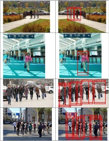
When analyzing the precision and recall, we can observe that some classifier has high precision but low recall and vice versa. When a classifier has high recall but low precision, it indicates that most of the positive images are correctly recognized but is also associated with a number of false positive. When a classifier has low recall but high precision, it indicates that we failed to detect most of the positive images but those predicted as positive are certainly positive. In such situation and also when the positive and negative datasets are not symmetric, it is preferred to go for F1 score. F1 score is a function of precision and recall, which is needed to have a balance between precision and recall. So, when comparing the F1 score of all classifiers from table 2, we observe that linear SVM has highest F1 score. The value of MCC lies between -1 and +1. A value of +1 indicates best prediction, 0 indicates average prediction and -1 indicates bad prediction. Among all classifiers in table 2, linear SVM has highest MCC. Youden’s index value lies between 0 and 1. A value of 1 indicates a perfect test. Observing table 2, youden’s index is highest for linear SVM. Miss rate and fall out are errors in prediction. So, a low value of both indicates perfect predictor. Observing table 2, we can see that fall out is lowest and miss rate is second lowest for linear SVM. All performance metrics in table 2 are obtained using a feature size of 4185. Using feature selectors, feature size is varied to obtain the best value of all these metrics. It is observed that using a feature size of 2100, performance of linear SVM and other classifiers is greatly enhanced. Table 3 provides the performance comparison of SVM classifier using mRMR feature selector. Table 4 provides the performance comparison of linear SVM using various feature selectors. Now, comparing the performance measures with and without feature selector from tables 2, 3 and 4, we can observe that accuracy is highest for linear SVM with mRMR feature selector (92.75 %) followed by JMI (92.42 %). It can be observed that F1 score is highest for linear SVM with mRMR (0.9072) which takes into account both precision and recall. MCC (0.8496) and youden’s index (0.8377) is also highest for linear SVM with mRMR which makes the system perfect for pedestrian detection. Table 5 provides the comparison of computation time required for testing 10 images using linear SVM classifier with and without mRMR feature selector. It can be observed that the computation time reduces by approx. 67 % with feature size reduction of approx. 50 %. Figure 4 gives the pedestrian detection output using proposed system.
Figure 4. Pedestrian detection results using proposed detection system
An improved pedestrian detection framework is proposed in this paper comprising HSG descriptor, linear SVM classifier and mRMR feature selector. The experiment is performed on MIT datasets. The accuracy and F1 score of the proposed system is improved by 3.93 % and 6.59 % respectively compared to detection system without mRMR feature selector. It is seen that using mRMR feature selector, the feature size get reduced by approximately 50 % which led to decrease in computation time by approximately 67 %. Thus the proposed pedestrian detection system is regarded as a better candidate for use in an advanced pedestrian detection system.
[1] Dollar P, Wojek C, Schiele B, Perona P. (2009). Pedestrian detection: A benchmark. In IEEE Conference on Computer Vision and Pattern Recognition 6: 304-311. https://doi.org/10.1109/CVPR.2009.5206631
[2] Benenson R, Omran M, Hosang J, Schiele B. (2015). Ten years of pedestrian detection, what have we learned? In Agapito L, Bronstein M, Rother C. (eds) Computer Vision - ECCV 2014 Workshops. ECCV 2014. Lecture Notes in Computer Science 8926. Springer. https://doi.org/10.1007/978-3-319-16181-5_47
[3] Bilal M, Khan A, Karim, Khan MU, Kyung C. (2017). A low-complexity pedestrian detection framework for smart video surveillance systems. IEEE Transactions on Circuits and Systems for Video Technology 27(10): 2260-2273. https://doi.org/10.1109/TCSVT.2016.2581660
[4] Lowe DG. (2004). Distinctive image features from scale-invariant keypoints. International Journal of Computer Vision. 60: 91-110. https://doi.org/10.1023/B:VISI.0000029664.99615.94
[5] Lowe DG. (1999). Object recognition from local scale-invariant features. In Proceedings of the Seventh IEEE International Conference on Computer Vision, Kerkyra, Greece, pp. 1150-1157. https://doi.org/10.1109/ICCV.1999.790410
[6] Bay H, Ess A, Tuytelaars T, Van L, (2008). Speeded-up robust features (SURF). Computer Vision and Image Understanding 110(3): 346–359. https://doi.org/10.1016/j.cviu.2007.09.014
[7] Mu Y, Yan S, Liu Y, Huang T, Zhou B. (2008). Discriminative local binary patterns for human detection in personal album. In Proceedings of the IEEE Conference on Computer Vision and Pattern Recognition, pp. 1-8. https://doi.org/10.1109/CVPR.2008.4587800
[8] Nanni L, Lumini A. (2008). Ensemble of multiple pedestrian representations. IEEE Transactions on Intelligent Transportation Systems 9: 365-369. https://doi.org/10.1109/TITS.2008.922882
[9] Ojala T, Pietikainen M, Harwood D. (1994). Performance evaluation of texture measures with classification based on kullback discrimination of distributions. In Proceedings of the 12th International Conference on Pattern Recognition 1: 582-585. https://doi.org/10.1109/ICPR.1994.576366
[10] Dalal N, Triggs B. (2005). Histograms of oriented gradients for human detection. In IEEE Computer Society Conference on Computer Vision and Pattern Recognition (CVPR'05) 1: 886-893. https://doi.org/10.1109/CVPR.2005.177
[11] Freeman WT, Roth M. (2013). Orientation histograms for hand gesture recognition. Presented at the IEEE Intl. Wkshp. on Automatic Face and Gesture Recognition, Zurich.
[12] Belongie S, Malik J, Puzicha J. (2002). Shape matching and object recognition using shape contexts. IEEE Transactions on Pattern Analysis and Machine Intelligence 24(4): 509-522. https://doi.org/10.1109/34.993558
[13] Viola P, Jones M. (2001). Rapid object detection using a boosted cascade of simple features. In Proceedings of the IEEE Computer Society Conference on Computer Vision and Pattern Recognition 1: 511-518. https://doi.org/10.1109/CVPR.2001.990517
[14] Heikkilä M, Pietikäinen M, Heikkilä J. (2004). A texture-based method for detecting moving objects. In 15th British Machine Vision Conference 1: 187-196. https://doi.org/10.5244/c.18.21
[15] Sankar R, Mishra RK. (2018). Outage probability analysis of selective-decode and forward cooperative wireless network overtime varying fading channels with node mobility and imperfect CSI condition. Proceedings of TENCON 2018: 0508-0513. https://doi.org/10.1109/TENCON.2018.8650275
[16] Ahonen T, Hadid A, Pietikäinen M. (2004). Face recognition with local binary patterns. European Conference on Computer Vision, Springer 3021: 469-481. https://doi.org/10.1007/978-3-540-24670-1_36
[17] Guo Z, Zhang L, Zhang D. (2010). Rotation invariant texture classification using LBP variance (LBPV) with global matching. Pattern Recognition 43(3): 706-719. https://doi.org/10.1016/j.patcog.2009.08.017
[18] Sachan V, Kumar I, Sankar R, Mishra RK. (2018). Analysis of transmit antenna selection based selective decode forward cooperative communication protocol. Traitement du Signal 35(1): 47-60. https://doi.org/10.3166/TS.35.47-60
[19] Liao S, Chung AC. (2007). Face recognition by using elongated local binary patterns with average maximum distance gradient magnitude. In 8th Asian Conference on Computer Vision, pp. 672-679. https://doi.org/10.1007/978-3-540-76390-1_66
[20] Wang X, Han TX, Yan S. (2009). An hog-lbp human detector with partial occlusion handling. In IEEE 12th International Conference on Computer Vision, pp. 32-39. https://doi.org/10.1109/iccv.2009.5459207
[21] Wei L, Bing Y, Chengwei D, Liying C, Huai Y, Hong Z. (2015). A pedestrian-detection method based on heterogeneous features and ensemble of multi-view-pose part. IEEE Transactions on Intelligent Transportation Systems 16: 813-824. https://doi.org/10.1109/TITS.2014.2342936
[22] Xin Y, Xiaosen S, Li S. (2011). A combined pedestrian detection method based on haar-like features and HOG feature. In Proceedings of the 3rd International Workshop on Intelligent Systems and Applications (ISA), pp. 1-4. https://doi.org/10.1109/ISA.2011
[23] Wojek C, Schiele B. (2008). A performance evaluation of single and multi-feature people detection. In Rigoll G. (eds) Pattern Recognition. DAGM 2008. Lecture Notes in Computer Science, 5096. Springer, Berlin, Heidelberg, pp. 82-91. https://doi.org/10.1007/978-3-540-69321-5_9
[24] Maji S, Berg AC, Malik J. (2008). Classification using intersection kernel support vector machines is efficient. In IEEE Conference on Computer Vision and Pattern Recognition. (CVPR), pp. 1-8. https://doi.org/10.1109/CVPR.2008.4587630
[25] Kumar I, Sachan V, Sankar R, Mishra RK. (2018). An investigation of wireless S-DF hybrid satellite terrestrial relaying network over time selective fading channel. Traitement du Signal 35(2): 103-120. https://doi.org/10.3166/ TS.35.103-120
[26] Wang P, Shen CH, Barnes N, Zheng H. (2012). Fast and robust object detection using asymmetric totally corrective boosting. IEEE Transactions on Neural Networks and Learning Systems 23: 33-46. https://doi.org/10.1109/TNNLS.2011.2178324
[27] Liu PX, Ni HY, Fu B, Bo F, Li WH, Wang Y, Wang SJ. (2014). Detection of partially occluded pedestrians by an enhanced cascade detector. Intelligent Transport Systems, IET 8: 621-630. https://doi.org/10.1049/iet-its.2012.0173
[28] Peng H, Long F, Ding C. (2005). Feature selection based on mutual information criteria of max-dependency, max-relevance, and min-redundancy. IEEE Transactions on Pattern Analysis and Machine Intelligence 27(8): 1226-1238. https://doi.org/1226-1238.10.1109/TPAMI.2005.159
[29] Mit pedestrian dataset. [Online]. http://cbcl.mit.edu/software-datasets/PedestrianData/, accessed on 20 April 2019.