Valerio D’Alessandro* | Matteo Falone | Renato Ricci
OPEN ACCESS
The main of aim this work is to enable a previously developed solver to computations involving turbulent flows. Hence, the flow field developing around a NACA 0012 at Re = 5 ∙ 104, M = 0.4, α = 5° is adopted as benchmark.
In this work we mainly address the correct definition of simulation settings in order to accurately capture the more relevant aerodynamic features of the aforementioned flow problem. Thus, all the results deriving from the iterative grid generation process are carefully described and discussed.
computational fluid dynamics, OpenFOAM, direct numerical simulation, compressible Navier-stokes equations
The long term goal of this research is to gain an insight of the sound emission produced by an isolated airfoil equipped with noise reduction devices [1]. In particular, our interest is devoted to the trailing edge serrations and to the physical mechanisms behind the possible sound emission reduction obtained using them. These phenomena are still not well understood, thus they deserve attention by our community and accurate numerical simulations are needed to achieve this goal. In the Computational Fluid-Dynamics (CFD) community it is well known that high resolution methods are strictly required in order to face Computational Aeroacoustics (CAA) problems, [2]. However, similar methods are typically adopted in academic codes with a very limited dissemination to the general public. That is why we have developed an open–source solver for the direct computation of the aeroacoustic sound. Our solver is based on OpenFOAM library which is actracting growing interest from CFD community [3, 4]. The solver development and its validation against laminar flows benchmarks are carefully described in a previously published paper [5]. Thus, one of the main aims of our ongoing work is to enable our CFD/CAA solver to turbulent flows computations. In this paper we present and discuss the results of the flow deriving from the direct computation of the flow field developing around a NACA 0012 airfoil at Re = 5 ∙ 104, M = 0.4, α = 5°.
Is worth noting that, for the considered configuration, a laminar separation bubble (LSB) is generated on the suction side. It extends for a wide-rage of the airfoil upper surface. Moreover, in the reattachment zone, a vortex shedding that convict up to the trailing edge is produced. Due to flow-field complexity this problem can be considered an appropriate benchmark for Direct Numerical Simulation (DNS) approaches [6-9]. Therefore, in this paper we conduct a campaign of numerical simulations aimed in the definition of the numerical settings suitable for the correct prediction of the aforementioned flow field. No particular care is here devoted to the acoustic fields prediction which is, differently, the matter of future developments.
This paper is organized as follows. Sec. 2 presents the governing equations considered here. Sec. 3 briefly describes the discretization technique. Sec. 4 is devoted to the numerical results and Sec. 5 contains the conclusions.
The flow model equations, based on the set of conservative variables read:
$\frac{\partial \psi }{\partial t}+\nabla \cdot {{\mathbf{F}}_{c}}(\psi )\nabla \cdot {{\mathbf{F}}_{v}}(\psi ,\nabla \psi )=\sigma \left( {{\psi }_{ref}}\text{ }\psi \right)$ (1)
where,
$\mathbf{\psi }={{\left( \rho ,\rho {{u}_{i}},\rho E \right)}^{T}}$ (2)
In Eq. (1) the convective and viscous fluxes, appearing in the right hand side, are evaluated in a standard way:
${{\mathbf{F}}_{\mathbf{c},j}}=\left( \begin{matrix} \rho {{u}_{j}} \\ \rho {{u}_{1}}{{u}_{j}}+p{{\delta }_{1j}} \\ \rho {{u}_{2}}{{u}_{j}}+p{{\delta }_{2j}} \\ \rho {{u}_{3}}{{u}_{j}}+p{{\delta }_{3j}} \\ \rho {{u}_{j}}H \\\end{matrix} \right)$, ${{\mathbf{F}}_{\mathbf{v},\text{j}}}=\left( \begin{matrix} 0 & {} \\ {{\tau }_{1j}} & {} \\ {{\tau }_{2j}} & {} \\ {{\tau }_{3j}} & {} \\ {{\tau }_{ji}}{{u}_{i}} & {{q}_{j}} \\\end{matrix} \right)$ (3)
It is also important to remark that the viscous stress tensor is computed using the constitutive relation for Newtonian fluids, while for heat flux vector the Fourier postulate is used:
${{\tau }_{ij}}=\mu \left( \begin{array}{*{35}{l}} \partial {{u}_{i}} \\ \partial {{x}_{j}} \\\end{array}+\begin{array}{*{35}{l}} \partial {{u}_{j}} & 2\partial {{u}_{k}} \\ \partial {{x}_{i}} & 3\partial {{x}_{k}} \\\end{array}{{\delta }_{ij}} \right),{{q}_{i}}=\lambda \begin{matrix} \partial T \\ \partial {{x}_{i}} \\\end{matrix}$ (4)
Moreover, the pressure is computed assuming the ideal gas equation of state as thermodynamic model, while the fluid temperature is evaluated starting from the total internal energy according to:
$p=\rho \left( \gamma \text{ 1} \right)\left( \begin{matrix} E & \begin{matrix} 1 \\ 2 \\\end{matrix} & {{u}_{k}}{{u}_{k}} \\\end{matrix} \right),\text{ }{{c}_{v}}T=E+\begin{matrix} \begin{matrix} 1 \\ 2 \\\end{matrix} & {{u}_{k}}{{u}_{k}} \\\end{matrix}$ (5)
The artificial term, in the right–hand side of Eq. (1), represent the expression of a sponge layer; it produces a damping of the flow variables near the external boundaries to a known reference solution. A detailed description of its implementation and sizing can be found in the ref. [5].
A collocated unstructured finite volume method, available within OpenFOAM library, is adopted to solve the governing equation. The kinetic energy conserving scheme of Pirozzoli, [6], was used for convective terms approximation. The adoption of a similar scheme is particularly attracting for scale resolving simulations due to its low dissipative properties. On the other hand, standard central schemes for diffusive contributions are used. For time integration a 2N storage explicit Runge–Kutta (ERK) scheme was implemented in order to exploit its good performance for large scale computations. In particular we have considered a five stage, fourth order accurate, ERK scheme available in the open literature [7]. In our computational experience this scheme is really appealing since it allows to use a maximum Courant number equal to 1. Thus, it allows to exploit good parallel behaviour of the explicit approaches without a severe time-step size restriction.
A particular mention has to be devoted to the computational grids which were generated using an in-house code developed by our group. The code was specifically developed for mesh generation problems involving arbitrary airfoils, and it enables multi-block structured grids to be obtained. C-type grids with far field boundaries placed at about 6 airfoil chors, c, were built. Furthermore, the sponge layer thickness is derived from the frequency of vortex shedding obtained after LSB reattachment. The total number of the grids’ cells employed in this work is reported in Table 1. It is worth noting that in all the previous cases the dimensioless height of the first cell next to the wall was set to 10-4.
Table 1. Computational mesh
|
Grid |
Number of Cells |
|
G1 |
1.789.860 |
|
G2 |
2.162.460 |
|
G3 |
2.421.900 |
In this section, we present our numerical results in terms of standard parameters relating to fluid dynamic fields, i.e. (i) drag and lift coefficients; (ii) pressure and skin friction coefficients.
The dimensionless drag and lift coefficients are given by Eq. (6):
${{C}_{D}}=\frac{2{{D}^{\prime }}}{\rho u_{\infty }^{2}c},{{C}_{L}}=\frac{2{{L}^{\prime }}}{\rho u_{\infty }^{2}c}$ (6)
On the contrary, pressure and skin friction coefficients are defined as follows:
${{c}_{p}}=\begin{matrix} 2\left( p\text{ }{{p}_{\infty }} \right) \\ \rho u_{\infty }^{2} \\\end{matrix},{{c}_{f}}=\begin{array}{*{35}{l}} 2{{\tau }_{w}} \\ \rho u_{\infty }^{2} \\\end{array}$ (7)
We want to remark that in the following we present time-averaged values of coefficients introduced in Eqns. (6) and (7).
The Strohual number, St, was also evaluated:
$\text{St}=\frac{fc}{{{u}_{\infty }}}$ (8)
All the solutions were obtained a MARCONI-100 HPC system hosted by CINECA. A good weak scalability was found up to 104 cells for each core; thus 256 CPU-core were used for the finest grid (G3).
4.1 NACA 0012 at Re = 5 ∙ 104, M = 0.4, α = 5°
In this subsection we describe all the main results deriving from the computations of the flow field around a NACA0012 airfoil at Re = 5 · 104, M = 0.4, α = 5°. The Prandtl number, Pr, is fixed equal to 0.75, while the dynamic viscosity derives from Sutherland equation. Note also that, in all the case here handled the dimensionless time-step size is 2 · 10-5.
A key element of the flows over airfoils at moderate Reynolds numbers can be found in the strong spanwise coherence of the pressure fluctuations [8]. Therefore, the investigation of the aeroacoustic field, produced by the interaction of an airfoil and the incoming flow, can be addressed through 2D DNS [8, 9]. Since, ultimately, our long term goal is related to aeroacoustic field prediction, in the following we will refer to 2D domains.
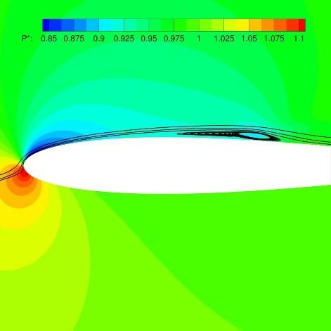
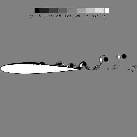
It is also very important to stress that, for the specific configuration of interest in this paper, a long LSB is generated on the suction side, see Figure 1. Furthermore, in the reattachment zone, a vortex shedding that convect up to the trailing edge is produced, as represented in Figure 2. The interaction between the above mentioned vortical structures and the airfoil trailing edge is commonly identified as one of the main aeroacoustic sound source [9]. Thus, it is very easy to understand that a variety of fluid phenomena are present and must be accurately resolved. For this reason the correct definition of grid resolution requirements for DNS of the flow around an airfoil at incidence is a challenging task. The iterative method of grid generation is mandatory for the current case, since a priori grid requirements are not known.
The Strohual number, related to the vortex shedding in the reattachment zone, is almost independent from the different grids here considered. Its value is 3.35 and it is in good agreement with literature references [8, 9].
On the contrary, looking a Table 2, is very clear that under-resolved force coefficients were obtained on our finest grid (G1). When the simulations were continued on grid G2 and G3 the mean lift coefficient increased notably. A good agreement between our results and literature ones [10], can be highlighted.
Figure 1. Time-averaged pressure coefficient and streamlines
Figure 2. Contour of the vorticity out of plane
Table 2. Time averaged force coefficients
|
Case |
CL |
CD |
|
Jones [10] |
0.499 |
0.0307 |
|
G1 |
0.4386 |
0.0313 |
|
G2 |
0.4619 |
0.0314 |
|
G3 |
0.4726 |
0.0316 |
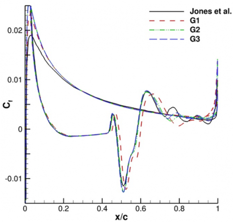
Figure 3. Time-averaged skin friction coefficient
In Figure 3 can be observed the time averaged skin friction coefficient, Cf, distribution computed along the airfoil surface. It is very interesting to note as the reattachment point, moves upstream if the grid resolution increases. This feature influences the wavy Cf distribution after the reattachment point. Globally, negligible differences are observed in CL and Cf coefficients between grids G2 and G3. In particular skin friction coefficient behaviour suffer a very slight impact in the region of secondary separation.
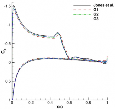
Time-averaged pressure coefficient, Cp, distributions are depicted in Figure 4 which illustrates the significant length of the pressure-plateau caused by the LSB. A local pressure minimum can be observed in proximity of the end of the pressure plateau which is, typically, identified as the transition point location. It is worth emphasizing that, the previous one, is a two-dimensional phenomenon which was already noted in similar cases [10] and also on flat plate simulations [11].
Figure 4. Time-averaged pressure coefficient
We want to put in evidence that in all the cases above discussed the time averaged aerodynamic coefficients are computed on time window ranging from 180 to 270 physical seconds.
Lastly, in our opinion G2 grid captures quite well the vortex shedding behaviour observed in two-dimensions, with no evidence of significant under-resolution.
In this paper we have presented our ongoing work on the direct computation of the flow developing around an airfoil in a turbulent flow. Indeed, our code, briefly presented here, was already extensively tested against laminar flow showing very good performance. Therefore, one of the main aims of the paper is related to evaluation of our approach against turbulent flows configurations. No particular care is here devoted to the acoustic fields prediction which is, differently, the matter of future developments.
The results, discussed in Sec. 4, have put in evidence as aerodynamic parameters are almost well predicted after an iterative grid generation strategy. This point was mandatory since no literature data are available in this sense. The selected benchmark problem was the NACA 0012 airfoil at Re = 5 · 104, M = 0.4, α = 5°. It is a quite challenging problem, since it reveals several critical issues. However, our computations seem to be sufficiently accurate to obtain a reliable prediction of the selected configuration.
Finally, this work can be considered a stepping stone to the open-source direct computation of the aeroacoustic field which develops around a rigid body in a turbulent flow.
We acknowledge the CINECA Award N. HP10B3UA3N YEAR 2019 under the ISCRA initiative, for the availability of high performance computing resources and support.
[1] Cappanera, G., D’Alessandro, V., Giammichele, L., Ricci, R. (2019). Acoustic investigation of aerodynamic appendages for wind turbine blades: Fluid-dynamic tests. TECNICA ITALIANA-Italian Journal of Engineering Science, 63(2-4): 329-335. https://doi.org/10.18280/ti-ijes.632-431
[2] Colonius, T., Lele, S.K. (2004). Computational aeroacoustics: Progress on nonlinear problems of sound generation. Progress in Aerospace sciences, 40(6): 345-416. https://doi.org/10.1016/j.paerosci.2004.09.001
[3] Arif, M.R., Hasan, N. (2020). Effect of thermal buoyancy on vortex-shedding and aerodynamic characteristics for fluid flow past an inclined square cylinder. International Journal of Heat and Technology, 38(2): 463-471. https://doi.org/10.18280/ijht.380223
[4] Borreani, W., Bruzzone, M., Chersola, D., Firpo, G., Lomonaco, G., Palmero, M., Panza, F., Ripani, M., Saracco, P., Viberti, C.M. (2017). Preliminary thermal-fluid-dynamic assessment of an ADS irradiation facility for fast and slow neutrons. International Journal of Heat and Technology, 35(1): S186-S190. https://doi.org/10.18280/ijht.35Sp0126
[5] D’Alessandro, V., Falone, M., Ricci, R. (2020). Direct computation of aeroacoustic fields in laminar flows: Solver development and assessment of wall temperature effects on radiated sound around bluff bodies. Computers & Fluids, 203: 104517. https://doi.org/10.1016/j.compfluid.2020.104517
[6] Pirozzoli, S. (2010). Generalized conservative approximations of split convective derivative operators. Journal of Computational Physics, 229(19): 7180-7190. https://doi.org/10.1016/j.jcp.2010.06.006
[7] Kennedy, C.A., Carpenter, M.H., Lewis, R.M. (2000). Low-storage, explicit Runge–Kutta schemes for the compressible Navier–Stokes equations. Applied Numerical Mathematics, 35(3): 177-219. https://doi.org/10.1016/S0168-9274(99)00141-5
[8] Sandberg, R.D., Jones, L.E., Sandham, N.D., Joseph, P.F. (2009). Direct numerical simulations of tonal noise generated by laminar flow past airfoils. Journal of Sound and Vibration, 320(4-5): 838-858. https://doi.org/10.1016/j.jsv.2008.09.003
[9] Sandberg, R., Jones, L., Sandham, N. (2008). Direct numerical simulations of noise generated by turbulent flow over airfoils. 14th AIAA/CEAS Aeroacoustics Conference (29th AIAA Aeroacoustics Conference), Vancouver, British Columbia Canada, pp. 2861. https://doi.org/10.2514/6.2008-2861
[10] Jones, L.E. (2008). Numerical studies of the flow around an airfoil at low Reynolds number. Doctoral Dissertation, University of Southampton.
[11] Pauley, L.L., Moin, P., Reynolds, W.C. (1990). The structure of two-dimensional separation. Journal of fluid Mechanics, 220: 397-411. https://doi.org/10.1017/S0022112090003317