B.J. Akinbo* | B.I. Olajuwon | I.A. Osinuga | S.I. Kuye
OPEN ACCESS
In this article, the significance of chemical reaction and thermo-diffusion in Walters’ B fluid is examined with medium porosity under the influence of non-uniform heat generation\absorption. The nonlinear ordinary differential equations describing the flow are obtained via similarity variables and tackled by Homotopy Analysis Method. The results show among others that involvement of chemical reaction contributes to the shrinking of concentration buoyancy effect while dimensionless temperature overshoot with large values of convective heat parameter and heat generation\absorption which enable thermal potency to gain entrance to the quiescent-fluid, indicating that the two parameters can be used for drying of the components.
Generation\Absorption, Chemical reaction, Thermo-diffusion, Similarity Variables, Homotopy Analysis Method (HAM)
The boundary layer transport over a vertical surface is an essential type of flow encountered in many engineering processes (See Vajravelu and Hadjinicolaou [1]) due to its daily applications in various sectors like boundary layer resistors in aerodynamics and fabrication of adhesive tapes e.t.c. The modeling of Newtonian fluid which has a perfect agreement with Navier Stoke equation has plays a significant role in modeling of several manufacturing process. However, the recent development in Science and Technology brings about the concept of Non-Newtonian fluid which also found to be an integral part of fluid mechanics to overcome low thermal conductivity of polymeric liquid among others. Hayat et al. [2] reported the opposite behaviors of temperature-field and concentration-field for thermal Biot number on convective flow of Magnetohydrodynamic Walters-B nanlfluid with variable thickness via a nonlinear stretching sheet. Sharma et al. [3] investigated stability of Walters’ (Model B′) type of stratified elastico-viscous fluid with horizontal magnetic strength and rotation in medium porosity. On the contrary to Newtonian type of fluids, the system is observed to be unstable on the account of stable stratification via small values assigned for permeability. Sharma and Rana [4] studied thermal instability through elastico-viscous-Walters' (Model B’) via rotation in medium porosity and variable gravity and pinpoint that Walters’ (model B’) acts like Newtonian model for stationary convection case. Similar case is reported through the two rotating viscoelastic superposed (Walters B') fluids by Kumar and Singh [5] and Makanda et al. [6] worked on free convection in the flow of viscoelastic model through a cone in a medium porosity with impact of viscous dissipation. Prakash et al. [7] examined Magnetohydrodynamic dusty viscoelastic (Walters’ liquid model-B) stratified type of fluid through a medium porosity with variable viscosity. Joneidi et al. [8] used Homotopy Analysis Method to investigate Walters’ B model fluid in a vertical channel via porous wall. Other researchers like [9-15].
Triggered by the previous effort in the literature with very little attentions on Walters’ B fluid under the influence of the convective boundary condition, this work is set to investigate the influence of chemical reaction and thermo-diffusion in an electrically conducting Walters’ B fluid over a vertical stretching-sheet, embedded in a porous medium with convective boundary condition. Walters’ B fluid is a subclass of non-Newtonian type of fluid that discloses the behaviors of various polymeric liquids encountered in chemical engineering and biotechnology among others
We consider a steady flow of an incompressible Walters’ B fluid over a vertical layer. The heat transfer analysis is executed with non-uniform heat generation\absorption while the mass transfer is considered with reaction rate and thermo diffusion effect. The layer wall is considered constant with temperature (and Concentration) T and C higher than the ambient temperature $T_{\infty}$(Concentration $C_{\infty}$) respectively. We assumed that the plated is heated by convection at temperature Tf which provides heat transfer coefficient hf. A magnetic field B0 of uniform strength is applied in y-direction. The magnetic reynold number is assumed to be very small, and so, the induced magnetic parameter is not taken account. The Joule heating effect is as well neglected as it really very small to slow the motion of free convection. x-axis is taken parallel to the direction of the flow and y-axis is normal to it (see Figure 1). The stretching sheet is moving with a velocity $u_{\mathrm{w}}(x)=a x$ and a>0.
Adopting the assumption expressed above, the two-dimensional Walters’ B model equation is given as (Mihra et al. [16])
$\frac{\partial u}{\partial x}+\frac{\partial v}{\partial y}=0$ (1)
$\begin{aligned} u \frac{\partial u}{\partial x}+v \frac{\partial u}{\partial y}=v & \frac{\partial^{2} u}{\partial y^{2}}-\frac{\sigma B_{0}^{2} u}{\rho}-\frac{v}{k} u \\ &-k_{0}\left[u \frac{\partial^{3} u}{\partial x \partial y^{2}}+v \frac{\partial^{3} u}{\partial y^{3}}+\frac{\partial u}{\partial x} \frac{\partial^{2} u}{\partial y^{2}}\right.\\ &\left.-\frac{\partial u}{\partial y} \frac{\partial^{2} u}{\partial x \partial y}\right] g \beta_{T}\left(T-T_{\infty}\right) \\ &+g \beta_{c}\left(C-C_{\infty}\right) \end{aligned}$ (2)
$u \frac{\partial T}{\partial x}+v \frac{\partial T}{\partial y}=\alpha \frac{\partial^{2} T}{\partial y^{2}}+Q_{0}$ (3)
$u \frac{\partial C}{\partial x}+v \frac{\partial C}{\partial y}=D_{m} \frac{\partial^{2} C}{\partial y^{2}}+\frac{D_{m} K_{T}}{T_{m}} \frac{\partial^{2} C}{\partial y^{2}}-r\left(C-C_{\infty}\right)$ (4)
with a suitable boundary condition slated as follows $u(x, 0)=$ $u_{\mathrm{w}}(x)=a x, v(x, 0)=0$
$-k \frac{\partial T(x, 0)}{\partial y}=h_{f}\left[T_{f}-T(x, 0)\right], \quad \mathrm{C}(x, 0)=C_{\mathrm{W}}$ (5)
$U(x, \infty)=0, \quad T(x, \infty)=T_{\infty}, \quad C(x, \infty)=C_{\infty}$ (6)
where $u$ and $v$ in the expression above, respectively denote the velocity components in $x$ and $y$ directions, $T_{m}$ is the mean fluid temperature, $Q_{0}$ is the non-uniform heat generation labsorption defined as $Q_{0}=\frac{k u_{\mathrm{w}}(x)}{\rho C_{p} x \mathrm{v}}\left[A\left(T-T_{\infty}\right) u+\right.$$\left.\left(T-T_{\infty}\right) B\right], \beta_{T}$ represents thermal expansion coefficient, $C_{p}$is the specific heat at constant pressure, while $v$ denotes kinematic viscosity, $\beta_{c}$ body forth concentration expansion coefficient, $D_{m}$ is the mass diffusivity, $\alpha$ represents thermal diffusivity while $\sigma$ is the fluid electrical conductivity, $g$ denotes acceleration due to gravity while $r$ typifies chemical rate coefficient and $\rho$ is the density.
On introducing the stream function $u=\frac{\partial \psi}{\partial y}$ and $v=-\frac{\partial \psi}{\partial x}$, the continuity equation (1) is automatically satisfied (Hashim et al. [17] and Narender et al. [18]). Applying the similarity variables defined by
$\eta=y \sqrt{\frac{a}{v}}, \quad \psi=x \sqrt{a v} f(\eta), \quad \theta(\eta)=\frac{T-T_{\infty}}{T_{f}-T_{\infty}}$, $\emptyset(\eta)=\frac{C-C_{\infty}}{C_{w}-C_{\infty}}$ (7)
On equations $(2-6),$ where $\eta$ represents the independent similarity variable $\theta(\eta)$ and $\emptyset(\eta),$ denote the temperature and concentration respectively, give the dimensionless Momentum, Energy and Concentration equations as follows
$\begin{aligned} \frac{d^{3} f}{d \eta^{3}}+f(\eta) \frac{d^{2} f}{d \eta^{2}}-&\left(\frac{d f}{d \eta}\right)^{2}-(M n+P s) \frac{d f}{d \eta} \\ &+\beta\left[\left(\frac{d^{2} f}{d \eta^{2}}\right)^{2}-2 \frac{d f}{d \eta} \frac{d^{3} f}{d \eta^{3}}\right.\\ &\left.+f(\eta) \frac{d^{4} f}{d \eta^{4}}\right]+\lambda_{T} \theta(\eta)+\lambda_{M} \emptyset(\eta) \\ &=0 \end{aligned}$ (8)
$\frac{d^{2} \theta}{d \eta^{2}}+\operatorname{Prf}(\eta) \frac{d \theta}{d \eta}+A \frac{d f}{d \eta}+B \theta(\eta)=0$ (9)
$\frac{d^{2} \emptyset}{d \eta^{2}}+S c f(\eta) \frac{d \emptyset}{d \eta}+S r \frac{d^{2} \theta}{d \eta^{2}}-R S c \emptyset(\eta)=0$ (10)
with
$f(\eta=0)=0, \frac{d f(\eta=0)}{\mathrm{d} \eta}=1$
$\frac{d \theta(\eta=0)}{\mathrm{d} \eta}=B i[\theta(\eta=0)-1]$ (11)
$\emptyset(\eta=0)=1$
$\frac{\partial f(\eta \rightarrow \infty)}{\partial \eta}=0, \quad \theta(\eta \rightarrow \infty)=0=\emptyset(\eta \rightarrow \infty)$ (12)
where $R=\frac{r}{a}$ body-forth rate of chemical reaction, $M n=\frac{\sigma B_{0}^{2}}{\rho a}$ is the magnetic field, $\beta=\frac{a k_{0}}{\mathrm{v}}$ is the Weissenberg Number, $P s=\frac{v}{K a}$ stands for porosity parameter, $\lambda_{T}=\frac{G r_{x}}{\left(\operatorname{Re}_{x}\right)^{2}}$ stands for thermal buoyancy parameter, while $\lambda_{M}=\frac{G c}{\left(\operatorname{Re}_{x}\right)^{2}}$ body forth mass buoyancy parameter, $G r_{x}=\frac{g \beta_{T}\left(T-T_{\infty}\right) x^{3}}{v^{2}}$ represents thermal Grashof Number while $G c_{x}=\frac{g \beta_{C}\left(T-T_{\infty}\right) x^{3}}{v^{2}}$ denotes solutal Grashof Number, $\operatorname{Re}_{x}=\frac{u(x)}{\mathrm{v}}$ is the Relyold Number, $\operatorname{Pr}=\frac{\mathrm{v} \rho \mathrm{Cp}}{k}$ is the prandtl number, $S c=\frac{\mathrm{r}}{D_{m}}$ is the Schmidtl number, $S r=\frac{K_{T}\left(T_{f}-T_{\infty}\right)}{T_{m}\left(C_{w}-C_{\infty}\right)}$ is the Soret number, and $B i=\frac{h_{f}}{k} \sqrt{\frac{v}{a}}$ connotes convective heat parameter. Owing to the engineering application of the study, the expression for skin friction coefficient, Local Nusselt number, and Local Sherwood number are respectively considered as
$\begin{aligned} R e_{x}^{\frac{1}{2}} C_{f}=(1-\beta) f^{\prime \prime}(0) & \\ & R e_{x}^{-\frac{1}{2}} N u=-\theta^{\prime}(0), R e_{x}^{-\frac{1}{2}} S h \\ &=-\emptyset^{\prime}(0) \end{aligned}$ (13)
Following Akinbo and Olajuwon $[19], \tau_{w}$ act as shear stress on the plate, $q_{w}$ body forth the surface while $q_{m}$ expresses the surface mass.
In solving nonlinear differential equation, many methods can be used, such as shooting techniques with Rung-kutta method, differential transformation method and so on. Homotopy Analysis Method is chosen over others, having standout as most efficient method in solving higher order nonlinear differential equations with both small and far field boundary conditions. In line with Hayat et’ al. [2], the initial guesses, which satisfies (11) and (12) are given by:
$f_{0}(\eta)=1-\exp (-\eta)$$\theta_{0}(\eta)=\frac{B i \exp (-\eta)}{(1+B i)}, \emptyset_{0}(\eta)$$=\exp (-\eta)$ (14)
and the auxiliary linear operations $L_{f}, L_{\theta}$, and $L_{\emptyset}$ which are respectively taken as:
$L_{f}[f(\eta ; r)]=\frac{\partial^{3} f(\eta ; r)}{\partial \eta^{3}}-\frac{\partial f(\eta ; r)}{\partial \eta}, L_{\theta}[\theta(\eta ; r)]$
$=\frac{\partial^{2} \theta(\eta ; r)}{\partial \eta^{2}}-\theta(\eta ; r) L_{\emptyset}[(\eta ; r)]$ (15)
$=\frac{\partial^{2} \emptyset(\eta ; r)}{\partial \eta^{2}}-\emptyset(\eta ; r)$
It agrees with the following properties:
$L_{f}\left[C_{1}+C_{2} \exp (\eta)+C_{3} \exp (-\eta)\right]=0$
$L_{\theta}\left[C_{4}+C_{5} \exp (-\eta)\right]$ (16)
$=0 L_{\emptyset}\left[C_{6}+C_{7} \exp (-\eta)\right]=0$
where $C_{1}, C_{2}, \ldots, C_{7}$ denote constants.
3.1 Zero-order deformation problem
$(1-r) L_{f}\left[f(\eta ; r)-f_{0}(\eta)\right]$$=r \hbar_{f} H_{f}(\eta) N_{f}[f(\eta ; r), \theta(\eta ; r), \emptyset(\eta ; r)]$ (17)
$(1-r) L_{\theta}\left[f(\eta ; r)-\theta_{0}(\eta)\right]$$=r \hbar_{A} H_{\theta}(\eta) N_{\theta}[f(\eta ; r), \theta(\eta ; r)]$ (18)
$(1-r) L_{\emptyset}\left[f(\eta ; r)-\emptyset_{0}(\eta)\right]$$=r \hbar_{\emptyset} H_{\emptyset}(\eta) N_{\emptyset}[f(\eta ; r), \theta(\eta ; r), \emptyset(\eta ; r)]$ (19)
here $\hbar \neq 0$ and $H \neq 0$ represent the auxiliary function and $r \in[0,1]$ is the embedded parameter, satisfying the following boundary conditions.
$\begin{aligned} f(\eta=0 ; r)=0, &\left.\frac{\partial f(\eta ; r)}{\partial \eta}\right|_{\eta=0}=1, \\ &\left.\frac{\partial \theta(\eta ; r)}{\partial \eta}\right|_{\eta=0} \\ &=B i[\theta(\eta=0 ; r)-1], \\ & \emptyset(\eta=0 ; r)=1 \end{aligned}$ (20)
$\begin{aligned}\left.\frac{\partial f(\eta ; r)}{\partial \eta}\right|_{\eta \rightarrow \infty}=& 0, \\ & \theta(\eta \rightarrow \infty ; r)=0=\emptyset(\eta \rightarrow \infty ; r) \end{aligned}$ (21)
where the $N_{f}, N_{\theta},$ and $N_{\emptyset}$ denote the nonlinear operator, expressed as
$\frac{\partial^{3} f(\eta ; r)}{\partial \eta^{3}}+f(\eta ; r) \frac{\partial^{2} f(\eta ; r)}{\partial \eta^{2}}-\left(\frac{\partial f(\eta ; r)}{\partial \eta}\right)^{2}$
$-(M n+P s) \frac{\partial f(\eta ; r)}{\partial \eta}+\lambda_{T} \theta(\eta ; r)+\lambda_{m} \emptyset(\eta ; r)$
$-\beta\left[\begin{array}{c}2 \frac{\partial f(\eta ; r)}{\partial \eta} \frac{\partial^{2} f(\eta ; r)}{\partial \eta^{2}} \\ -f(\eta ; r) \frac{\partial^{4} f(\eta ; r)}{\partial \eta^{4}}-\left(\frac{\partial^{2} f(\eta ; r)}{\partial \eta^{2}}\right)^{2}\end{array}\right]=0$ (22)
$\frac{\partial^{2} \theta(\eta ; r)}{\partial \eta^{2}}+\operatorname{Pr} \frac{\partial \theta(\eta ; r)}{\partial \eta} f(\eta ; r)+A \frac{\partial f(\eta ; r)}{\partial \eta}$
$+B \theta(\eta ; r)=0$ (23)
$\frac{\partial^{2} \emptyset(\eta ; r)}{\partial \eta^{2}}+\operatorname{Scf}(\eta ; r) \frac{\partial \emptyset(\eta ; r)}{\partial \eta}+\operatorname{sr} \frac{\partial^{2} \theta(\eta ; r)}{\partial \eta^{2}}$$-\operatorname{RSc} \emptyset(\eta ; r)=0$ (24)
Applying $r=0$ and $r=1$, we respectively have the following solution from equation (17)-(19).
$L_{f}\left[f(\eta ; 0)-f_{0}(\eta)\right]=0,$$\quad L_{\theta}\left[\theta(\eta ; 0)-\theta_{0}(\eta)\right]$$\quad=0, \quad L_{\emptyset}\left[\emptyset(\eta ; 0)-\emptyset_{0}(\eta)\right]$$\quad=0$ (25)
$f(\eta ; 0)=f_{0}(\eta), \quad \theta(\eta ; 0)=\theta_{0}(\eta)$$\emptyset(\eta ; 0)=\emptyset_{0}(\eta)$ (26)
with
$\begin{aligned} f(\eta=0 ; 0)=0, & \frac{\partial f(\eta=0 ; 0)}{\partial \eta}=1 \\ & \frac{\partial \theta(\eta=0 ; 0)}{\partial \eta} \\ &=B i[\theta(\eta=0 ; 0)-1] \\ & \emptyset(\eta=0 ; 0)=1 \end{aligned}$ (27)
$\begin{aligned} \frac{\partial f(\eta \rightarrow \infty ; 0)}{\partial \eta}=0 &, \theta(\eta \rightarrow \infty ; 0)=0 \\ &=\emptyset(\eta \rightarrow \infty ; 0) \end{aligned}$ (28)
$0=N_{f}[f(\eta ; r), \theta(\eta ; r), \emptyset(\eta ; r)], 0$$=N_{\theta}[f(\eta ; r), \theta(\eta ; r)],$$\quad 0=N_{\emptyset}[f(\eta ; r), \emptyset(\eta ; r)]$ (29)
But $\hbar_{f}, H_{f}(\eta) \neq 0, \hbar_{\theta} H_{\theta}(\eta) \neq 0$ and $\hbar_{\emptyset} H_{\emptyset}(\eta) \neq 0$
$f(\eta ; 1)=f(\eta), \quad \theta(\eta ; 1)=\theta(\eta), \emptyset(\eta ; 1)=\emptyset(\eta)$ (30)
with
$\begin{aligned} f(\eta=0 ; 1)=0, & \frac{\partial f(\eta=0 ; 1)}{\partial \eta} \\ &=1, \frac{\partial \theta(\eta=0 ; 1)}{\partial \eta} \\ &=B i[\theta(\eta=0 ; r)-1], \emptyset(\eta\\ &=0 ; 1)=1 \end{aligned}$ (31)
$\frac{\partial f(\eta \rightarrow \infty ; 1)}{\partial \eta}=0, \theta(\eta \rightarrow \infty ; 1)=0$$=\emptyset(\eta \rightarrow \infty ; 1)$ (32)
When $r$ rise from zero to one, the function $f(\eta ; r), \theta(\eta ; r)$ and $\emptyset(\eta ; r)$ tends to $f_{0}(\eta), \theta_{0}(\eta)$ and $\emptyset_{0}(\eta)$ to be solutions $f(\eta), \theta(\eta)$ and $\emptyset(\eta) .$ By the application of Taylor series,
$\begin{aligned} f(\eta ; r)=f_{0}(\eta)+& \sum_{m=1 \atop \theta(\eta ; r)}^{\infty} f_{m}(\eta) r^{m}, \\ &=\theta_{0}(\eta)+\sum_{m=1 \atop \infty}^{\infty} \theta_{m}(\eta) r^{m} \quad \emptyset(\eta ; r) \\ &=\emptyset_{0}(\eta)+\sum_{m=1}^{\infty} \emptyset_{m}(\eta) r^{m} \end{aligned}$ (33)
where
$f_{m}(\eta)=\frac{1}{m !} \frac{\partial^{m} f(\eta ; r)}{\partial \eta^{m}}$$\theta_{m}(\eta)$
$\quad=\frac{1}{m !} \frac{\partial^{m} \theta(\eta ; r)}{\partial \theta^{m}},$ and $\emptyset_{m}(\eta)$
$=\frac{1}{m !} \frac{\partial^{m} \emptyset(\eta ; r)}{\partial \emptyset^{m}}$
The convergence of the series (33) is subject to the auxiliary parameter $\hbar$. Assuming $\hbar$ is chosen such that the series (33) converge at $r=1,$ we have
$f(\eta)=f_{0}(\eta)+\sum_{m=1}^{\infty} f_{m}(\eta),$
$\theta(\eta)=\theta_{0}(\eta)+\sum_{m=1}^{\infty} \theta_{m}(\eta),$
$\varnothing(\eta)=\emptyset_{0}(\eta)+\sum_{m=1}^{\infty} \emptyset_{m}(\eta)$ (34)
The mth-order deformation are expressed as
$L_{f}\left[f_{m}(\eta)-\chi_{m} f_{m-1}(\eta)\right]$
$\quad=\hbar R_{m}^{f}(\eta), L_{\theta}\left[\theta_{m}(\eta)\right.$
$\left.\quad-\chi_{m} \theta_{m-1}(\eta)\right]$
$\quad=\hbar R_{m}^{\theta}(\eta) L_{\emptyset}\left[\emptyset_{m}(\eta)\right.$
$\left.\quad-\chi_{m} \emptyset_{m-1}(\eta)\right]=\hbar R_{m}^{\emptyset}(\eta)$ (35)
$\begin{aligned} f_{m}(\eta=0 ; r)=0 & \frac{\partial f_{m}(\eta=0 ; r)}{\partial \eta}=0, \\ & \frac{\partial \theta_{m}(\eta=0 ; r)}{\partial \eta} \\ &=B i\left[\theta_{m}(\eta=0 ; r)\right], \\ &=0 ; r)=0 \end{aligned}$ (36)
$\begin{aligned} \frac{\partial f_{m}(\eta \rightarrow \infty ; r)}{\partial \eta}=& 0, \\ & \theta_{m}(\eta \rightarrow \infty ; r)=0 \\ &=\emptyset_{m}(\eta \rightarrow \infty ; r) \end{aligned}$ (37)
where,
$R_{m}^{f}(\eta)$$=\frac{d^{3} f_{m-1}(\eta)}{d \eta^{3}}-(M n+P s) \frac{d f_{m-1}(\eta)}{d \eta}$$+\sum_{n=0}^{m-1} f_{n}(\eta) \frac{d^{2} f_{m-1-n}(\eta)}{d \eta^{2}}$
$-\sum_{n=0}^{m-1} \frac{d f_{n}(\eta)}{d \eta} \frac{d f_{m-1-n}(\eta)}{d \eta}$$-\beta\left[\begin{array}{l}2 \sum_{n=0}^{m-1} \frac{d f_{n}(\eta)}{d \eta} \frac{d^{2} f_{m-1-n}(\eta)}{d \eta^{2}}- \\ \sum_{n=0}^{m-1} f_{n}(\eta) \frac{d^{4} f_{m-1-n}(\eta)}{d \eta^{4}}- \\ \sum_{n=0}^{m-1} \frac{d^{2} f_{n}(\eta)}{d \eta^{2}} \frac{d^{2} f_{m-1-n}(\eta)}{d \eta^{2}}\end{array}\right]+\lambda_{T} \theta_{m-1}(\eta)$$+\lambda_{M} \emptyset_{m-1}(\eta)$ (38)
$R_{m}^{\theta}(\eta)=\frac{d^{2} \theta_{m-1}(\eta)}{d \eta^{2}}+\operatorname{Pr} \sum_{n=0}^{m-1} f_{n}(\eta) \frac{d \theta_{m-1-n}(\eta)}{d \eta}$
$+A \frac{d f_{m-1}(\eta)}{d \eta}+Q \theta_{m-1}$ (39)
$R_{m}^{\emptyset}(\eta)=\frac{d^{2} \emptyset_{m-1}(\eta)}{d \eta^{2}}+S c \sum_{n=0}^{m-1} f_{n}(\eta) \frac{d \emptyset_{m-1-n}(\eta)}{d \eta}$
$+\operatorname{Sr} \frac{d^{2} \theta_{m-1}(\eta)}{d \eta^{2}}-R S c \emptyset_{m-1}(\eta)$ (40)
and $\chi_{m}=0$ for $m \leq 1, \chi_{m}=1$ for $m>1$
Therefore, the general solutions of equation (35) are
$f_{m}(\eta)=f_{m}^{*}(\eta)+C_{1}+C_{2} \exp (-\eta)+C_{3} \exp (\eta)$ (41)
$\theta_{m}(\eta)=\theta_{m}^{*}(\eta)+C_{4}+C_{5} \exp (\eta)$ 422)
$\emptyset_{m}(\eta)=\emptyset_{m}^{*}(\eta)+C_{6}+C_{7} \exp (\eta)$ (43)
3.2 Convergence of the HAM solution
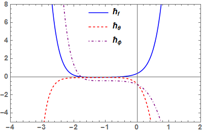
Figure 2. $\hbar_{f}, \hbar_{\theta}, \hbar_{\emptyset}$ -curves for $f^{\prime \prime}(0), \theta^{\prime}(0)$ and $\emptyset^{\prime}(0)$
respectively
Following Liao [20], Hayat et al. [21] and Akinbo and Olajuwon [19, 22] suggestions, the non-zero auxiliary parameters $\hbar_{f}, \hbar_{\theta}$ and $\hbar_{\varnothing}$ play a pivotal role in controlling the convergence region of the series solution. On introducing $A=$ $0.01, B=0.01, \beta=0.1, M n=1, P s=1, \lambda_{T}=0.1, \lambda_{M}=$ 0.1, $\operatorname{Pr}=0.72, S c=0.62,$ Sr $=0.1, B i=0.1$ and $R=0.1$ we have the admissible values of $\hbar_{f}, \hbar_{\theta}$ and $\hbar_{\emptyset}$ which are presented at a region where $\hbar-$ curve becomes parallel, such as $-1.8 \leq \hbar_{f} \leq-0.4,-1.5 \leq \hbar_{\theta} \leq-0.5$ and $-2.1 \leq \hbar_{\emptyset} \leq-0.4$ (See Figure (2)).
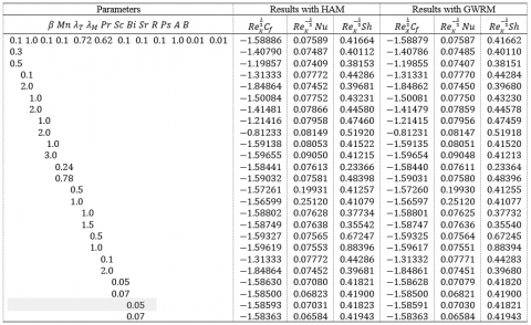
Table 1. Computational results for the Skin-friction coefficient, Local Nusselt number and Local Sherwood number/Validation with Galerkin Weighted Residual Method (GWRM)
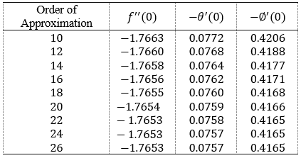
Table 2. The convergence of iterations
Figure 3. Behavours of Mn on Velocity f'(η)
In this section, the behaviors of various parameters encountered are discussed by holding A=0.01, B=0.01, β=0.1, Mn=1, Ps=1, λT=0.1, λM=0.1, Pr=0.72, Sc=0.62, Sr=0.1, Bi=0.1 and R=0.1, constant for each varying parameter.
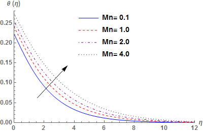
Figure 4. Behavours of Mn on Temperature θ(η)
Figures 3-4 illustrate the effect of Magnetic field (Mn) on velocity and temperature profiles. From Figure 3, we observed that increase in Mn improve the magnetic interaction and electric field which pioneer retarding force called Lorentz force that act against the flow and reduces the motion of the fluid and its layer thickness. However, the opposite phenomenon is observed on fluid temperature as higher values of Mn enhances the temperature distribution across the layer due to the frictional heating produced within the boundary layer. This in turns increases thermal boundary layer thickness
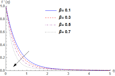
Figure 5. Behaviours of β on Velocity f'(η)
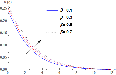
Figure 6. Behaviours of β on Temperature θ(η)
Figures 5-6 depict the behaviours of Weissenberg number β on Velocity and Temperature profiles. It is observed from Figure 7 that increase in β slow down the velocity distribution across the layer which in tuns lower its boundary layer thickness. The physics behind this reduction corresponds to the large values of β which pioneer viscoelasticity through the tensile stresses that consequently reduce the motion of the fluid. However, reverse phenomenon is observed on temperature profile (See Figure 6).
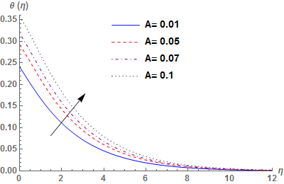
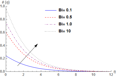
Figures 7-8 presents the influence of generation\absorption (A,B) on temperature profile. As expected, increase in (A,B) magnifies temperature effect across the boundary which overshoot the temperature profile to its peak values and suddenly fall monotonically to the free stream zero value far away from the plate surface agreeing with the far field boundary conditions, thereby strengthen the thermal boundary layer thickness. However, similar behaviour is observed on temperature profile (See Figure 9) due to the interaction of convective heat parameter (Bi). This justifies that higher values of Bi stimulates more convective heating across the boundary layer which in turns increases the operating temperature (and boundary layer thickness) and enable the thermal effect to penetrate to the quiescent fluid.
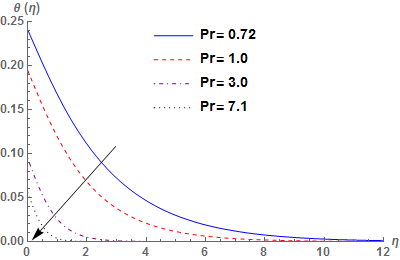
Figure 10 is plotted to show the effect of prandtl number (Pr) on temperature profile. Increase in Pr owing to the low thermal diffusivity enhances the conducting process higher than the convection, which ultimately lower the molecular motion of which its aftermath effect reduces fall the temperature distribution across the boundary layer and lower its layer thickness. This reveals that at smaller values of Pr, the fluid possesses higher thermal diffusivity. Figure 11 depicts the physical behaviours of Schmidtl number (Sc) on concentration profiles. Higher values of Sc as a result of low molecular diffusivity, suppresses the diffusion properties of the fluid, which ultimately reduces the concentration profile and declines concentration boundary layer thickness.
Figure 7. Behavours of A on Temperature θ(η)
Figure 8. Behaviours of B on Temperature θ(η)
Figure 9. Behaviours of Bi on Temperature θ(η)
Figure 10. Behaviours of Pr on Temperature θ(η)
Figure 11. Behaviours of Sc on Concentration ∅(η)
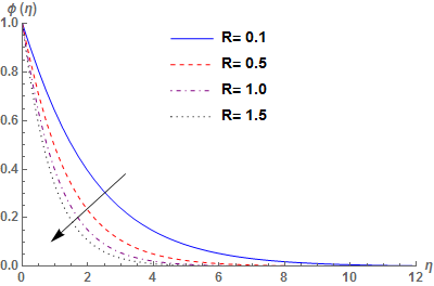
Figure 12. Behaviours of R on Concentration ∅(η)
The effect of chemical reaction parameter (R) on concentration profile is presented in Figure 12. It is noticed that higher values of R pioneers greater Shrinking on concentration buoyancy effect which consequently declines concentration profile and lower its layer thickness.
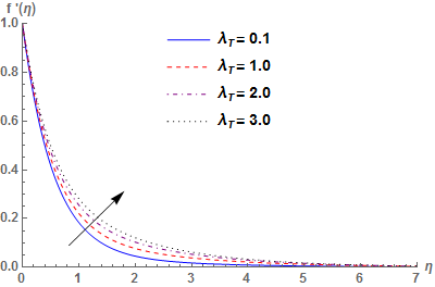
Figure 13. Behaviours of λ_T on Velocity f'(η)
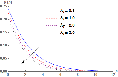
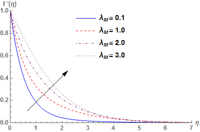
Figures 13-14 exhibit the behaviors of thermal buoyancy parameter (λ_T) on velocity temperature profiles and concentration profiles while the mass buoyancy parameter ( λ_M) is reported in Figures 15-16 for velocity and concentration profile respectively. The higher values of (λ_T,λ_M) accelerate the motion of the fluid maximize the fluid velocity (and its layer thickness). However, opposite phenomenon are observed on temperature and concentration profiles which respectively decline thermal and concentration boundary layers thicknesses. These results agreed with the expectation as λ_T>0 contributes to the cooling of the surface and λ_M>0 shows a greater concentration at the plate surface than free stream concentration.
Figure 14. Behaviours of λ_T on Temperature θ(η)
Figure 15. Behaviours of λ_M on Velocity f'(η)
Figure 16. Behaviours of λ_M on Concentration ∅(η)
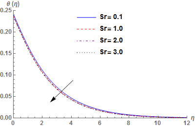
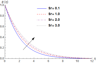
Figures 17-18 presents the effect of Soret number (Sr) on temperature and concentration profiles. Physically, we observed from Figure 17 that increase in Sr contribute to the cooling of the surface which ultimately reduces the thermal boundary layer thickness. However, concentration boundary layer thickness declines due to the opposite phenomenon observed on concentration profile (See Figure 18).
Figure 17. Behavours of Sr on Temperature θ(η)
Figure 18. Behaviours of Sr on Concentration ∅(η)
Figure 19. Behaviours of Ps on Velocity f'(η)
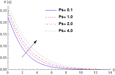
The effect of porosity parameter (Ps) on velocity and temperature profiles are presented in Figures 19-20. Increase in Ps causes a greater resistance to the flow and slow down the movement of the fluid particles which ultimately reduces the momentum boundary layer thickness. The interactions of Ps>0 pioneer heating within the layer that consequently boosts thermal boundary layer thickness.
Figure 20. Behaviours of Ps on Temperature θ(η)
From Table 1, HAM and GWRM are in good concordat in comparison. It is obvious from the table that almost all values of skin-friction coefficient $R e_{x}^{\frac{1}{2}} C_{f}$ demonstrated negative, indicating weaker movement of the flow due to the drag forces on the surface. However, the local Nusselt number $R e_{x}^{\frac{1}{2}} Nu$ Nu and Sherwood number $R e_{x}^{\frac{1}{2}} Sh$ improves for higher values of (λT,λM). This in turns strengthen the rate of heat and mass transfer with an opposite result as Weissenberg number (β), Magnetic Parameter (Mn), Soret number (Sr) and Prandtl number (Pr) gain strength. It is also observed from the table that rate of heat transfer experienced a greater boost for large values of Biot number (Bi) with a similar phenomenon on rate of mass transfer as Schmidtl number (Sc) and Reaction rate parameter (R) increases. Table 2 presents the convergence of the iteration with the far field boundary condition. It can be seen from the table that momentum and concentration equations converge at 22th-order while the energy equation converges at 24th-order of iterations.
In this paper, HAM is presented at 20th-order of approximation to solve the governing equations describing the interaction of chemical reaction and thermo-diffusion in a hydromagnetic Walters’ B fluid. The choice of 20th-order is to meet the far field boundary condition and the behaviors of embedded parameter are discussed accordingly through graph and table with the following conclusions drawn from the results obtained.
A space-dependent heat generation/absorption
B temperature-dependent heat generation/absorption
$\beta$ Weissenberg number
Mn Magnetic field parameter
Ps porosity parameter
Pr prandtl number
Sr Soret number
R Reaction rate parameter
$\lambda_{T}$ Thermal buoyancy parameter
$\lambda_{M}$ Mass buoyancy parameter
Sc Schmidt number
Bi convective heat parameter
$\beta_{T}$ thermal expansion coefficient
$\beta_{c}$ concentration expansion coefficient
Cp specific heat at constant pressure
Dm mass diffusivity
$\alpha$ thermal diffusivity
g acceleration due to gravity
Cf Surface drag force
Nu Nusselt number
Sh Sherwood number
kT Thermal diffusion ratio
Tm Mean fluid temperature
Greek symbols
$\eta$ Similarity variable
$\alpha$ thermal diffusivity
$\psi$ Stream function
v kinematic viscosity
$\sigma$ fluid electrical conductivity
$\rho$ fluid density
[1] Vajravelu, K., Hadjinicolaou, A. (1998). Nonlinear hydromagnetic convection at a continuous moving surface. Nonlinear Analysis: Theory, Methods & Applications, 31(7): 867-882. https://doi.org/10.1016/S0362-546X(97)00444-6
[2] Hayat, T., Qayyum, S., Alsaedi, A., Ahmad, B. (2017). Magnetohydrodynamic (MHD) nonlinear convective flow of Walters-B nanofluid over a nonlinear stretching sheet with variable thickness. International Journal of Heat and Mass Transfer, 110: 506-514. https://doi.org/10.1016/j.ijheatmasstransfer.2017.02.082
[3] Sharma, V., Gupta, U. (2006). Stability of stratified elastico-viscous Walters'(Model B') fluid in the presence of horizontal magnetic field and rotation in porous medium. Archives of Mechanics, 58(2): 187-197.
[4] Sharma, V., Rana G.C. (2001). Thermal instability of a Walters' (Model B’) elastico-viscous fluid in the presence of variable gravity field and rotation in porous medium. J. Non-Equilib. Thermodyn, 26(1): 31-40.
[5] Kumar, P., Singh, M. (2007). Instability of two rotating viscoelastic (Walters B') superposed fluids with suspended particles in porous medium. Thermal Science, 11(1): 93-102. https://doi.org/10.2298/TSCI0701093K
[6] Makanda, G., Makinde, O.D., Sibanda, P. (2013). Natural convection of viscoelastic fluid from a cone embedded in a porous medium with viscous dissipation. Mathematical Problems in Engineering. https://doi.org/10.1155/2013/934712
[7] Prakash, O., Kumar, D., Dwivedi, Y.K. (2012). Heat transfer in MHD flow of dusty viscoelastic (Walters’ liquid model-B) stratified fluid in porous medium under variable viscosity. Pramana, 79(6): 1457-1470. https://doi.org/10.1007/s12043-012-0344-z
[8] Joneidi, A.A., Domairry, G., Babaelahi, M. (2010). Homotopy analysis method to Walter’s B fluid in a vertical channel with porous wall. Meccanica, 45(6): 857-868. https://doi.org/10.1007/s11012-010-9295-y
[9] Kumar, P. (1999). Stability of two superposed viscoelastic (Walters B') fluid-particle mixtures in porous medium. Zeitschrift für Naturforschung A, 54(5), 343-347. https://doi.org/10.1515/zna-1999-0511
[10] Sharma, R.C., Kumar, P. (1997). Study of the stability of two superposed Walters’(Model B’) visco-elastic liquids. Czechoslovak Journal of Physics, 47(2): 197-204. https://doi.org/10.1023/A:1021069730348
[11] Sunil, D., Sharma, R.C., Chand, S. (2000). Thermosolutal convection in Walter's (model B') fluid in porous medium in hydromagnetics. Studia Geotechnica et mechanica, 22(3-4): 3-14.
[12] Ali, F., Saqib, M., Khan, I., Sheikh, N.A. (2016). Application of Caputo-Fabrizio derivatives to MHD free convection flow of generalized Walters’-B fluid model. The European Physical Journal Plus, 131(10): 1-10. https://doi.org/10.1140/epjp/i2016-16377-x
[13] Bariş, S. (2002). Steady flow of a Walter's B'viscoelastic fluid between a porous elliptic plate and the ground. Turkish Journal of Engineering and Environmental Sciences, 26(5): 403-418.
[14] Thirumurugan, K., Vasanthakumari, R. (2016). Double-diffusive convection of non-Newtonian Walters’(MODELB’) viscoelastic fluid through brinkman porous medium with suspended particles. International Journal of Heat and Technology, 34(3): 357-363. https://doi.org/10.18280/ijht.340302
[15] Thirumurugan, K., Vasanthakumari, R. (2014). Hydromagnetics instability of non-Newtonian Walters' B'viscoelastic rotating fluid in porous medium. World Journal of Engineering, 11(4): 365-372. ISSN: 1708-5284
[16] Mishra, S.R., Baag, S., Bhatti, M.M. (2018). Study of heat and mass transfer on MHD Walters B′ nanofluid flow induced by a stretching porous surface. Alexandria Engineering Journal, 57(4): 2435-2443. https://doi.org/10.1016/j.aej.2017.08.007
[17] Hamid, A., Khan, M., Khan, U. (2018). Thermal radiation effects on Williamson fluid flow due to an expanding/contracting cylinder with nanomaterials: dual solutions. Physics Letters A, 382(30): 1982-1991. https://doi.org/10.1016/j.physleta.2018.04.057
[18] Narender, G., Manjula, N., Govardhan, K., Rajashekar, M.N. (2019). Heat and mass transfer of Williamson nanofluid with the effects of viscous dissipation and chemical reaction. TECNICA ITALIANA-Italian Journal of Engineering Science, 63(1): 108-113. https://doi.org/10.18280/ti-ijes.630115
[19] Akinbo, B.J., Olajuwon, B.I. (2019). Homotopy analysis investigation of heat and mass transfer flow past a vertical porous medium in the presence of heat source. International Journal of Heat and Technology, 37(3): 899-908. https://doi.org/10.18280/ijht.370328
[20] Liao, S.J. (2003). An analytic approximate technique for free oscillations of positively damped systems with algebraically decaying amplitude. International Journal of Non-Linear Mechanics, 38(8): 1173-1183. https://doi.org/10.1016/S0020-7462(02)00062-8
[21] Hayat, T., Shehzad, S.A., Alsaedi, A. (2012). Soret and Dufour effects on magnetohydrodynamic (MHD) flow of Casson fluid. Applied Mathematics and Mechanics, 33(10): 1301-1312. https://doi.org/10.1007/s10483-012-1623-6
[22] Akinbo, B.J., Olajuwon, B.I. (2019). Heat and mass transfer in magnetohydrodynamics (MHD) flow over a moving vertical plate with convective boundary condition in the presence of thermal radiation. Sigma: Journal of Engineering & Natural Sciences/Mühendislik ve Fen Bilimleri Dergisi, 37: 1031-1053.