Gangadharappa Sarthi*![]() | Naveena Chikkaguddaiah
| Naveena Chikkaguddaiah![]() | Manjunath Aradhya V. N.
| Manjunath Aradhya V. N.![]()
© 2023 IIETA. This article is published by IIETA and is licensed under the CC BY 4.0 license (http://creativecommons.org/licenses/by/4.0/).
OPEN ACCESS
An aberrant cell disorder called cancer/tumor causes uncontrollably dividing abnormal cells that eventually destroy body tissue. One type of cancer brought on by the unchecked expansion of malignant cells in the brain is the brain tumour. Future prognosis and treatment planning depend on accurate tumour segmentation and classification. Manual segmentation of brain tumor extent from 3D MRI volumes is a very time-consuming task and the performance is highly relied on operator’s experience. In this context, a reliable fully automatic segmentation method for the brain tumor segmentation is necessary for an efficient measurement of the tumor extent. In this study, we propose a fully automatic method for brain tumor segmentation, which is developed using U-Net based deep convolutional networks. Our method was evaluated on Multimodal Brain Tumor Image Segmentation datasets, which contain 110 high-grade brain tumor and 54 low-grade tumor cases. Cross validation has shown that our method can obtain promising segmentation efficiently.
U-net, CNN architecture, ReLU activation function
When aberrant cells develop out of control, infiltrate nearby tissues, and/or spread to other organs, it results in cancer, which can start at any particular part of our body, it may be on tissue also which lies in broad category of disease. Changes in the DNA sequence of important genes known as cancer genes cause abnormal behaviour in cancer cells. Therefore, all forms of cancer are inherited illnesses. Brain tumours can develop directly from brain tissue or they can attack brain from different body parts (metastasis). One of the deadliest cancer type is still brain lesion. The specific cell-intrinsic and micro environmental characteristics of brain tissues are thought to have a role in these tumours' capacity to withstand practically all traditional and new treatments. In 2020, it is predicted that the new cases would rise up to 19.2 million. Of these 9.3 would be related to men and 8.4 related to female. The whole body, from head to toe, is affected by several different types of cancer. There are almost 200 different forms of cancer, each with its own causes, signs, and therapies. Men are more likely to develop lung, colorectal, prostate, liver cancer and stomach than women, who are more likely to develop lung, breast, cervical, thyroid cancer and colorectal. The greatest crude incidence rate of cancer was found in Kerala, where there were 135.3 cases per 100,000 people. It is estimated that 16.4M tumor related deaths and 29.5 million new cases of chemo related diseases per year by the end of 2040.
One of the prevalent disorders of the neurological system, brain tumours have a serious negative impact on human health and can even be fatal. Among intracranial tumours, gliomas have the greatest death and morbidity rates. The two main types are high-grade glioma (HGG) and low-grade glioma (LGG) and individuals whose HGG has progressed typically have a two-year life expectancy. Numerous methods, including Positron Emission Tomography (PET), Magnetic Resonance imaging (MRI), Single-photon Emission Computed Tomography and Computed Tomography (CT) have been used to investigate brain malignancies (SPECT). The most popular methods for searching for brain illnesses are magnetic resonance imaging (MRI) and computed tomography (CT) and. If there is a brain tumour, these scans will nearly always reveal it.
A non-invasive imaging method known as magnetic resonance imaging (MRI) produces three-dimensional, intricate anatomical images. It is frequently used in the early diagnosis, monitoring, and compound for tumour.
Simulation and detection in alteration in the rotational axis of protons which are present in hydrogen leads to formation of biological tissues are resolved based on cutting edge technology. Due to its benefits of good soft tissue contrast, multi-parameter, imaging in any direction, non-invasive imaging, etc., MRI has emerged as the primary imaging technology for the solution and aid for glial cell cancer. Additionally, MRI can be used to obtain multiple of modalities, including T1-weighted with contrast enhancement (T1c), T2-weighted (T2), T1-weighted (T1) and Fluid Attenuated Inversion Recovery (FLAIR) [1], Different MRI techniques concentrate on various fine details of pictures and depict the features of brain tumours from various angles. For the purpose of making a medical diagnosis, organising a surgery, and developing a treatment plan, it is crucial to accurately segment brain tumours. Separating tumour tissues, such as necrosis, edoema, non enhancing core, and enhancing core, from normal brain tissues, such as the white matter (WM), grey matter (GM), and cerebrospinal fluid, is particularly important (CSF). However, accurately segmenting them is a very difficult problem, mostly for the reasons listed below. First of all, gliomas can differ widely from patient to patient in terms of shape, location, appearance, and size. Second, the border is usually hazy because gliomas frequently infect neighbouring tissues. Third, the issue is further exacerbated by the noise and image distortion brought on by many elements, such as imaging instruments or acquisition techniques. Every year, 40,000–50,000 people in India receive a brain tumour diagnosis [2]. Children make up 20% of this group, however this percentage was just around 5% up until a year ago. The goal of the Brain Tumor Segmentation (BraTS) challenge is to assess cutting-edge techniques for the fractionlization of brain tumours in multi-parametric magnetic resonance imaging (mpMRI) data. Since its creation, it has served as both a publicly accessible raw data and a standard test data. Pre-operative multi-institutional mpMRI scans are used in BraTS, which focuses on the fractions of gliomas, which are inherently diverse (in visual, form, and cytology) brain tumours. Additionally, BraTS 2018 concentrates on the survival rate of tumored person by integrated analysis of radiomic characteristics and machine learning (ML) algorithms so that it matches with the practical values of fractionlisation part. The datasets are well utilised for this research come from the BraTS Dataset. These datasets span from year to year and continuously include more upgraded photos. The BraTS 2015 raw data, for instance, is a metadata for segmenting images of brain tumours. There are 54 low grade gliomas (LGG) and 220 high grade gliomas (HGG) in the collection. T1, T1c, T2, and T2FLAIR are the four MRI modalities. Four intra-tumoral classes—puffy part in brain, augment tumour, non-augment tumour, and expiration—are provided as segmented "ground truth." Similar to BraTS 2017, BraTS 2018 is a raw data that provides complex 3D brain MRIs and accurate brain tumour fraction that have been annotated by medical professionals. Each case includes 4 MRI modalities (T1, T1c, T2, and FLAIR). The augment tumor, the peritumoraledoema, and the necrotic and non-enhancing tumour core are the three tumour subregions that are annotated. Three nested sub regions were created from the annotations: augment tumour (AT), tumour core (TC), and total tumour (WT) (ET). Using a variety of MRI scanners, the data were gathered from 19 different universities. Brain tumor therapy has major challenge like planning, the quantitative assessment, and establishment of tumor extent and accurate presentation of tumor from MR Images. It is a must to plan and monitor the progression of tumor. It is tedious and time consuming if manual delineation of brain tumor and expert hand is required to do manually. Hence an automated method for segmentation is proposed which helps large clinical facilities.
Yang and Song [3] proposed a U-net model-based automatic brain tumour image segmentation technique for magnetic resonance imaging (MRI). A U-net guideline model along with the ideal parameter form that is appropriate for fraction task is built using samples enhancement, reason for loss, and developement technique. Gobhinath et al. [4] explained that the three stages of image preprocessing, image segmentation and image morphological function are necessary for the identification of brain tumours.
Akram and Usman [5] explained brain tumour growth can be detected using magnetic resonance (MR) scans, using Filtering Techniques. Jemimma andVetharaj [6] explained captivating tonality imaging for the preferred image modality for evaluating brain tumours, and segmentation. Wulandari et al. [7] suggested that the watershed approach is used to mark the parts of the brain and those outside of it, and the cropping method is used to clean the skull. Brain tumours and brain tissues are contrasted in the segmentation results. Solomon et al. [8] described a semi-automated technique for segmenting and tracking the volume of brain tumours. MRI images are processed using a pipeline approach in this method. Bhandari et al. [9] described that a model to segment the brain MRI using CNN.
Zhang et al. [10] proposed a study which will concurrently points on implementation and unused units into U-Net for improvement towards presentation of brain tumor fractions which is peer to peer network using residual U-Net (AResU-Net). AlI et al. [11] proposed a substantial yet simple combinative method that produces more precise predictions by combining two segmentation networks—a 3D CNN and a U-Net. Ramya and Jayanthi [12] suggested segmenting any sort of brain data, Image distributed multilocation graph via kernel plotting is utilized. Singh et al. [13] explained the three stages of the diagnosis approach which includes segmentation, feature extraction, and preprocessing of magnetic resonance images.
Menze et al. [14] reported the design and outcomes of the MICCAI 2012 and 2013 conferences' joint Multimodal BRATS Benchmark project. Pitchai et al. [15] suggested segmenting the tumour site, a Fuzzy K-means method and an Artificial Neural Network have been combined. It has four stages: removing background noise, selecting and extracting attributes, classifying data, and segmenting data. Wang et al. [16] suggested to separate multi-modal magnetic resonance imaging (MR) pictures of brain tumours into backdrop and 3 graded regions—the overall lesion, the tumour nucleus, and the augmented tumour core—a cataract of fully convolutional neural networks is presented. Prastawa et al. [17] initially came up with a strategy that divides brain tumour and edoema into two phases. They start by making a reliable evaluation by the place and scattering of the normal magnitude bunches in the brain tissue.
Murugavalli and Rajamani [18] implemented the work that presents a neuro-fuzzy fractioning method for MRI data to identify different cells, including white matter, grey matter, CSF, and malignancy. Jayadevappa et al. [19] suggested to segment the brain tumour, a hybrid fractionation method combining GVF snake and marker-controlled watershed is used. The suggested approach is validated using actual MR images. Popuria et al. [20] introduced a variational approach to segmenting brain tumours.
Deng et al. [21] focused on image segmentation, which is cause for processing medical images. On the basis of geographical data and the fuzzy c-means algorithm, a new method for segmenting medical images is suggested. Corso et al. [22] suggested the mathematical formula for including soft model assignments in the previously model-free calculation of affinities.
Torrents-Barrena et al. [23] explored 3D encoder-decoder designs by utilising patch-based methods to save memory and lessen. Colman et al. [24] explained lesion segmentation in brain MRIs using a 2D deep residual Unet with 104 convolutional layers (DR-Unet104). Murthy and Sadashivappa [25] used various methods that been devised to find and separate the brain tumour. Effective brain tumour segmentation is accomplished via beginning and semantic techniques. Rezaei et al. [26] an autonomous peer-to-peer trainable architecture for the BraTS 2017 challenge that can segment heterogeneous brain tumours. Based on deep learning methods.
Shaikh et al. [27] proposed the use of an opaquely connected FCNN combined with processing after employing a DCR. Havaei et al. [28] introduced a fully autonomous DNN-based brain tumour fraction technique (DNNs). The suggested networks are designed to fit the low- and high-grade glioblastomas shown in MRI. Zeineldin et al. [29] presented a brand-new general deep learning architecture called Deep Seg for completely automated brain lesion identification and segmentation in FLAIR MRI data. Haghighi et al. [30] explained a semantic genesis to study conotationally high in presence via locating by itself, categorization by itself, and fixing by itself of the undemeath images of medical related 3D model that uses deep models.
A detailed literature survey has been made in the areas of MRI brain image preprocessing, segmentation, feature extraction and classification. It is clear from the literature survey, brain tumor Segmentation need to be enhanced with regard to the recognition rate, accuracy and precision.
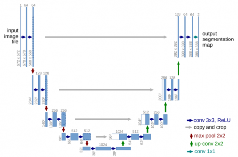
Among the available CNN, U-Net, with its U-shaped encoder-decoder structure. It segments the images by down-sampling and up-sampling using the original images and take outthe feature map that is similar to its actual type of image. Unet consists of two path contaracting and expanding path. U-Net is intended to be useful in the delineations needed for radiation treatment planning because it is distinguished by integrating both local features and general location information of the object. Even with a large number of samples, Unet can still produce relatively acceptable results. Both a 2D and a 3D format can be used to construct it, and both has benefits and drawbacks. In the 2D approach, the Unet planning can be practiced with pair of input-output 2D portion; a fractional architecture can be fed by any 3D sub volume by replacing all the 2D operations with equivalent 2D operations for 3D approach.
Figure 1. 3D-UNet architecture
An accuarate 3D Unet extension is accomplished by Unet only. The 3D Unet authorizes to proceed in 3D sub volume and receive an output for each graphical information of 3D space in the volume that specifies the expectation of a tumour. 2D convolutions produce a single image by applying the same weights throughout the entire depth of the stack of frames (many channels). In order to preserve the temporal information of the frame stack, 3D convolutions employ 3D filters and result in a 3D volume. The 3D direction of information is lessened with 2D U-Net since each image is treated separately as shown in Figure 1. This system, however, is capable of learning from several samples.
The 3D direction of information is enriched while the number of samples is reduced in 3D U-Net, increasing the quantity of information per sample. Semantic segmentation involves labelling each pixel in an image or voxel in a 3D volume. Because 3D unet offers the best segmentation for brain tumour subregions in MRI modalities, we thus tried semantic segmentation of MRI image using 3D Unet. It is made up of a contractive (encoder path) and expanding (decoder path) that uses convolution and pooling to build a bottleneck in the middle of the path.
Convolutions and up-sampling are used to recreate the image after this bottleneck. The 3D u-net segmentation presents a network and test approach which is based on the application of data enlargement to the given images, which is more effective, as part of the deep convolution neural network. A contacting path is used to capture circumstances, and a balancing growing path is used for exact localization. To categorise labels, a convolutional neural network (CNN)-based architecture is frequently utilised.
But more than just classification should be the goal in medical imaging. It ought to contain the localization, which is set up to foretell the class label of each pixel using the context of its immediate surroundings as input. The context of the image is captured via the encoder path. It is merely a stack of maximum pooling and convolutional layers. The depth is increased as the image size is gradually decreased by the encoder. This basically means that while learning the "WHERE" information in the image, the network forgot to learn the "WHAT" information. The encoder network performs the function of a feature extractor by using a sequence of encoder blocks to learn an conceptual representation of the input image.
Set of two 3x3 convolutions are formed as one block which follows a rectified Linear Unit (ReLU) a activation function. This function (ReLU) adds nonlinearity to the network, assisting in the generalization of training data. The associated decoder block is the skip connection for the output of ReLU. Following the ReLU activation function comes the dropout function. By deleting (ignoring) a few randomly selected neurons, it compels the network to learn a new representation. Neurons will become independent with the help of network. In turn, this promotes generalisation and prevents overfitting in the network. Then, a 2×2 max-pooling is used to cut the structural dimensions (height and width) of the feature maps in half.
The bridge completes the information flow by connecting the encoder and decoder networks. It consists of two 33-convolutional layers, with a ReLU activation function placed after each. The size steadily grows while the depth gradually lowers, and the decoder path is used to provide precise localisation. A semantic segmentation mask is produced from the abstract representation using the decoder network. Starting with a 2×2 transpose convolution, the decoder block is activated. It is then joined with the relevant skip connection feature map for the encoder block. These skip connections offer functionality that were occasionally lost owing to network depth.
Two 3×3 convolutions are utilised after that, and each is followed by a ReLU activation function. The final decoded output is subjected to 1×1 convolutions with sigmoid activation. The pixel wise classification is represented by masked segmentation which is created by sigmoid activation function.
As a result, this network is entirely convolutional from beginning to end. To retrieve the "WHERE" information, the decoder gradually uses up-sampling (precise localization). We concatenate the output of the transposed convolution layers with the feature maps from these encoders in order to leverage skip connections at each stage of the decoder to achieve more precise positioning. These skip connections give the decoder additional data, enabling it to produce more precise semantic characteristics.
They also act as a shortcut connection, enabling gradients to pass undegradedly to lower layers. Skip connections, to put it simply, increase the gradient flow during backpropagation, enabling the network to learn better representation. After each concatenation, we apply two consecutive regular convolutions so that the model can learn to put together a more precise result. Due to the size, complexity, and memory requirements of a full MRI scan, we are unable to offer one for training. As a result, we standardise the data and generate random sub volumes. The image we utilise has the size 128×128×128×3, but the input image has the dimensions 256×256×256×3. As a result, the size will vary from the original at various spots, but the essential element will stay the same.
In this section, segmentation by Wrapper based GA using CNN is discussed. Asequence of 30 images of FLAIR as well as T2 (23 abnormal & 7 normal) were considered in the performance assessment, out of these 95 objects were utilized in training and 30 objects were utilized in testing phase. The outcome is analyzed in terms of specificity, accuracy, Absolute Volume Measurement Error (AVME) and figure of merit(s). In this work, we compare proposed work with SVM.
The specificity of proposed Wrapper based GA using SVM segmentation and existing FCM based segmentation for both T2 and FLAIR images is shown in Table 1 of Specificity.
Table 1. Statistical comparison for the FLAIR, T2 input in terms of specificity
|
|
FLAIR |
T2 |
||
|
Data |
SVM (%) |
CNN (%) |
SVM (%) |
CNN (%) |
|
1 |
98.5923 |
99.5838 |
96.8602 |
99.8839 |
|
2 |
99.0007 |
99.6829 |
96.8856 |
99.9491 |
|
3 |
98.9668 |
99.6765 |
96.7296 |
99.9671 |
|
4 |
99.2618 |
99.6969 |
96.5252 |
99.9400 |
|
5 |
99.5206 |
99.8522 |
96.3061 |
99.9940 |
|
6 |
99.5148 |
99.8343 |
96.2331 |
99.9970 |
|
7 |
99.5210 |
99.7590 |
96.1287 |
99.9910 |
|
8 |
99.4670 |
99.8163 |
95.9441 |
99.9910 |
|
9 |
99.1225 |
99.5867 |
958313 |
99.8952 |
|
10 |
98.8796 |
95.7276 |
95.7276 |
99.9522 |
Table 2 gives a statistical comparison in terms of accuracy for Wrapper based GA using SVM segmentation and FCM. Experimental results show that GA based SVM method gives an accuracy of 99.25 % for FLAIR and 98.28 % for T2whereas FCM of 98.67% for FLAIR and 97.16 % for T2. This result shows the proficiency of Wrapper based GA using SVM segmentation in term of accuracy.
Table 2. Statistical comparison for the multimodality input image in terms of Accuracy
|
|
FLAIR |
T2 |
||
|
Data |
SVM (%) |
CNN (%) |
SVM (%) |
CNN (%) |
|
1 |
98.9641 |
98.5851 |
96.1458 |
98.9554 |
|
2 |
98.5966 |
98.9178 |
93.7037 |
98.4983 |
|
3 |
98.4635 |
98.8831 |
93.4549 |
98.4086 |
|
4 |
98.5532 |
99.0278 |
93.0787 |
98.2002 |
|
5 |
98.4722 |
99.1811 |
92.4132 |
97.9080 |
|
6 |
98.7847 |
99.1609 |
92.4016 |
98.0874 |
|
7 |
98.7500 |
99.1175 |
92.3264 |
98.1424 |
|
8 |
98.6921 |
99.0654 |
92.1991 |
98.0150 |
|
9 |
98.5793 |
98.8831 |
92.5926 |
98.1800 |
|
10 |
98.7355 |
98.7355 |
92.7112 |
97.9514 |
Table 3. Statistical comparison of multimodality input image in terms of time elapsed
|
|
FLAIR |
T2 |
||
|
Data |
SVM(Sec) |
CNN(Sec) |
SVM(Sec) |
CNN(Sec) |
|
1 |
0.10644 |
0.687467 |
0.247004 |
0.463591 |
|
2 |
0.10334 |
0.701177 |
0.072135 |
0.231283 |
|
3 |
0.095835 |
0.683585 |
0.080558 |
0.254667 |
|
4 |
0.108671 |
0.652442 |
0.104623 |
0.329427 |
|
5 |
0.107736 |
0.960127 |
0.074604 |
0.243118 |
|
6 |
0.13356 |
0.980784 |
0.075599 |
0.236125 |
|
7 |
0.103878 |
0.740483 |
0.079258 |
0.311487 |
|
8 |
0.093298 |
0.819494 |
0.072311 |
0.226894 |
|
9 |
0.096376 |
0.677372 |
0.106921 |
0.248339 |
|
10 |
0.100872 |
0.699691 |
0.081979 |
0.242185 |
Table 4. Volume measurement analysis for FCM and SVM
|
Data |
SVM (pixels) |
CNN (pixels) |
|
1 |
18432 |
27007 |
|
2 |
14679 |
9232 |
|
3 |
29742 |
22821 |
|
4 |
7623 |
11453 |
|
5 |
18789 |
3271 |
|
6 |
13654 |
22732 |
|
7 |
12957 |
6437 |
|
8 |
29394 |
13480 |
|
9 |
6327 |
8282 |
|
10 |
18432 |
27007 |
Table 3 gives the statistical comparison of FLAIR and T2 images, in terms of time elapsed. From table it understand the time taken by SVM is less then CNN for both T2 and FLAIR. Table 4 and Table 5 give the analysis of volumetric measurement in terms of automatic and absolute volume segmentation for the two methods SVM and CNN. From both tables we can understand that the volume varies in both methods. It’s obtained negative using absolute segmentation. Figure of merit for the two approaches is shown in Table 6. From table we can understand that SVM gives less merit when compare to CNN. The Volumetric analysis of manual and automatic segmentation of multimodality images is shown in Table 7. Here we compare CNN, SVM with manual and automatic segmentation. Volume varies with both the methods and with manual segmentation for 5 different data with FLAIR and T2.
Table 5. Comparative analysis of volume measurement for FCM, SVM of absolute segmentation
|
Data |
SVM (pixels) |
CNN (pixels) |
|
1 |
-17.35 |
21.102 |
|
2 |
20.093 |
-24.47 |
|
3 |
-2.11 |
-24.889 |
|
4 |
-21.27 |
18.292 |
|
5 |
76.754 |
-69.229 |
|
6 |
-38.77 |
1.9326 |
|
7 |
6.0051 |
-47.337 |
|
8 |
-3.255 |
-55.633 |
|
9 |
-34.65 |
-14.46 |
|
10 |
-17.35 |
21.102 |
Table 6. Statistical comparison of input images in terms of figure of merit
|
Data |
SVM |
CNN |
|
1 |
0.788978 |
0.82651 |
|
2 |
0.755297 |
0.799067 |
|
3 |
0.751111 |
0.978903 |
|
4 |
0.817083 |
0.787337 |
|
5 |
0.307714 |
0.232455 |
|
6 |
0.980674 |
0.61226 |
|
7 |
052663 |
0.939949 |
|
8 |
0.443669 |
0.967449 |
|
9 |
0.855402 |
0.653481 |
|
10 |
0.134055 |
0.477234 |
Table 7. Volumetric analysis for multimodality image
|
Image |
Data |
Manual Segmentation method |
Automatic segmentation |
Absolute volume measurement |
||
|
Type |
SVM |
CNN |
SVM |
CNN |
||
|
FLAIR |
1 |
22301 |
18432 |
27007 |
-17.35 |
21.102 |
|
2 |
12223 |
14679 |
9232 |
20.093 |
-24.47 |
|
|
3 |
30383 |
29742 |
22821 |
-2.11 |
-24.88 |
|
|
4 |
9682 |
7623 |
11453 |
-21.27 |
18.292 |
|
|
5 |
10630 |
18789 |
3271 |
76.754 |
-69.22 |
|
|
T2 |
6 |
22301 |
13654 |
22732 |
-38.77 |
1.932 |
|
7 |
12223 |
12957 |
6437 |
6.005 |
-47.33 |
|
|
8 |
30383 |
29394 |
13480 |
-3.255 |
-55.63 |
|
|
9 |
9682 |
6327 |
8282 |
-34.65 |
-14.46 |
|
|
10 |
10630 |
16187 |
1425 |
52.277 |
-86.59 |
|
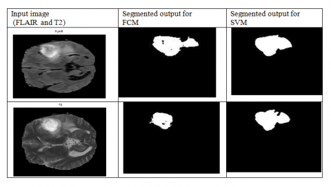
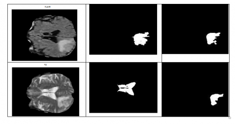
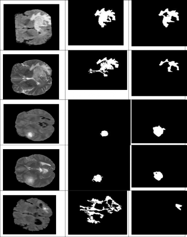
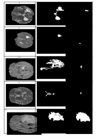
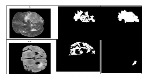
In Figure 2, the first column represents the multimodality input image (FLAIR and T2), the second column shows the segmented output image by using FCM algorithm and the third column represents the segmented output image by wrapper based GA using CNN. Here we can observe that detection brain tumor by both the methods for some samples. In some samples we can observe that misidentification. Hence the overall efficiency of the proposed system is proven. The segmented image shown in figure shows the efficiency of Wrapper based GA using CNN with SVM. The reduced computational time enhances the chance for of Wrapper based GA using a CNN algorithm to be used in the diagnosis of tumors. Hence this Wrapper based GA algorithm to be superior with the existing EM and level set and SVM.
Figure 2. First Column shows the input image of T2 and FLAIR, second coloumn shows the final segment output for FCM for T2 and FLAIR image and third coloumn shows the final segmented output for Wrapper based GA using SVM for T2 and FLAIR image
A brain tumour is an unanticipated mass of flesh where unchecked cell growth and multiplication occurs. These days, it is a widespread and grave issue. The complicated structure of tumours, including their size, form, and existence, makes it challenging to make the correct diagnosis of a brain tumour. Radiologists may make mistakes when manually detecting brain tumours, and their findings may differ from one another. This does not always imply a correct diagnosis. As a result, brain tumour detection requires some form of automation. When analysing medical images, image processing is crucial. Segmenting brain tumours is a technique for separating healthy brain tissue from aberrant tumour tissue. Different segmentation strategies have been addressed, along with the benefits and drawbacks of each. A thorough analysis of the work done by researchers to automate the task of segmenting and detecting brain tumours is presented. The ease of use and level of human involvement determine whether a given segmentation approach is clinically accepted.
[1] Somasundaram, S., Gobinath, R. (2019). Current trends on deep learning models for brain tumor segmentation and detection–A review. In 2019 International conference on machine learning, big data, cloud and parallel computing (COMITCon), pp. 217-221. https://doi.org/10.1109/COMITCon.2019.8862209
[2] Lather, M., Singh, P. (2020). Investigating brain tumor segmentation and detection techniques. Procedia Computer Science, 167: 121-130. https://doi.org/10.1016/j.procs.2020.03.189
[3] Yang, T., Song, J. (2018). An automatic brain tumor image segmentation method based on the U-Net. In 2018 IEEE 4th International Conference on Computer and Communications (ICCC), Chengdu, China, pp. 1600-1604. https://doi.org/10.1109/CompComm.2018.8780595
[4] Gobhinath, S., Anandkumar, S., Dhayalan, R., Ezhilbharathi, P., Haridharan, R. (2021). Human brain tumor detection and classification by medical image processing. In 2021 7th International Conference on Advanced Computing and Communication Systems (ICACCS), Coimbatore, India, pp. 561-564. https://doi.org/10.1109/ICACCS51430.2021.9441877
[5] Akram, M.U., Usman, A. (2011). Computer aided system for brain tumor detection and segmentation. In International conference on Computer networks and information technology, Abbottabad, Pakistan, pp. 299-302. https://doi.org/10.1109/ICCNIT.2011.6020885
[6] Jemimma, T.A., Vetharaj, Y.J. (2018). Watershed algorithm based DAPP features for brain tumor segmentation and classification. In 2018 International Conference on Smart Systems and Inventive Technology (ICSSIT), Tirunelveli, India, pp. 155-158. https://doi.org/10.1109/ICSSIT.2018.8748436
[7] Wulandari, A., Sigit, R., Bachtiar, M.M. (2018, October). Brain tumor segmentation to calculate percentage tumor using MRI. In 2018 International Electronics Symposium on Knowledge Creation and Intelligent Computing (IES-KCIC), Bali, Indonesia, pp. 292-296. https://doi.org/10.1109/KCIC.2018.8628591
[8] Solomon, J., Butman, J.A., Sood, A. (2004). Data driven brain tumor segmentation in mri using probabilistic reasoning over space and time. In Medical Image Computing and Computer-Assisted Intervention–MICCAI 2004: 7th International Conference, Saint-Malo, France, September 26-29, 2004. Proceedings, Part I 7, pp. 301-309. https://doi.org/10.1007/978-3-540-30135-6_37
[9] Bhandari, A., Koppen, J., Agzarian, M. (2020). Convolutional neural networks for brain tumour segmentation. Insights into Imaging, 11(1): 1-9. https://doi.org/10.1186/s13244-020-00869-4
[10] Zhang, J., Lv, X., Zhang, H., Liu, B. (2020). AResU-Net: Attention residual U-Net for brain tumor segmentation. Symmetry, 12(5): 721. https://doi.org/10.3390/sym12050721
[11] Ali, M., Gilani, S.O., Waris, A., Zafar, K., Jamil, M. (2020). Brain tumour image segmentation using deep networks. Ieee Access, 8: 153589-153598. https://doi.org/10.1109/ACCESS.2020.3018160
[12] Ramya, R., Jayanthi, K.B. (2012). Multiregion image segmentation by graph cuts for brain tumour segmentation. In Advances in Communication, Network, and Computing: Third International Conference, CNC 2012, Chennai, India, February 24-25, 2012, Revised Selected Papers 3, pp. 329-332. https://doi.org/10.1007/978-3-642-35615-5_51
[13] Singh, N., Das, S., Veeramuthu, A. (2017). An efficient combined approach for medical brain tumour segmentation. In 2017 International Conference on Communication and Signal Processing (ICCSP), Chennai, India, pp. 1325-1329. https://doi.org/10.1109/ICCSP.2017.8286598
[14] Menze, B.H., et al. (2014). The multimodal brain tumor image segmentation benchmark (BRATS). IEEE transactions on medical imaging, 34(10): 1993-2024. https://doi.org/10.1109/TMI.2014.2377694
[15] Pitchai, R., Supraja, P., Victoria, A.H., Madhavi, M. (2021). Brain tumor segmentation using deep learning and fuzzy K-means clustering for magnetic resonance images. Neural Processing Letters, 53: 2519-2532. https://doi.org/10.1007/s11063-020-10326-4
[16] Wang, G., Li, W., Ourselin, S., Vercauteren, T. (2018). Automatic brain tumor segmentation using cascaded anisotropic convolutional neural networks. In Brainlesion: Glioma, Multiple Sclerosis, Stroke and Traumatic Brain Injuries: Third International Workshop, BrainLes 2017, Held in Conjunction with MICCAI 2017, Quebec City, QC, Canada, September 14, 2017, Revised Selected Papers 3, pp. 178-190. https://doi.org/10.1007/978-3-319-75238-9_16
[17] Prastawa, M., Bullitt, E., Ho, S., Gerig, G. (2003). Robust estimation for brain tumor segmentation. In Medical Image Computing and Computer-Assisted Intervention-MICCAI 2003: 6th International Conference, Montréal, Canada, November 15-18, 2003. Proceedings 6, pp. 530-537. https://doi.org/10.1007/978-3-540-39903-2_65
[18] Murugavalli, S., Rajamani, V. (2007). An improved implementation of brain tumor detection using segmentation based on neuro-fuzzy technique. Journal of Computer Science, 3(11): 841-846. https://doi.org/10.3844/JCSSP.2007.841.846
[19] Jayadevappa, D., Kumar, S.S., Murty, D.S. (2009). A hybrid segmentation model based on watershed and gradient vector flow for the detection of brain tumor. International Journal of Signal Processing, Image Processing and Pattern Recognition, 2(3): 29-42.
[20] Popuri, K., Cobzas, D., Jagersand, M., Shah, S.L., Murtha, A. (2009). 3D variational brain tumor segmentation on a clustered feature set. In Medical Imaging 2009: Image Processing, 7259: 562-571. https://doi.org/10.1117/12.811029
[21] Deng, W., Xiao, W., Pan, C., Liu, J. (2009). MRI brain tumor segmentation based on improved fuzzy c-means method. In MIPPR 2009: Medical Imaging, Parallel Processing of Images, and Optimization Techniques, 7497: 677-682.https://doi.org/10.1117/12.832577
[22] Corso, J.J., Yuille, A., Sicotte, N.L., Toga, A.W. (2007). Detection and segmentation of pathological structures by the extended graph-shifts algorithm. In Medical Image Computing and Computer-Assisted Intervention–MICCAI 2007: 10th International Conference, Brisbane, Australia, October 29-November 2, 2007, Proceedings, Part I 10, pp. 985-993. https://doi.org/10.1007/978-3-540-75757-3_119
[23] Torrents-Barrena, J., Piella, G., Masoller, N., Gratacós, E., Eixarch, E., Ceresa, M., Ballester, M.Á.G. (2019). Segmentation and classification in MRI and US fetal imaging: recent trends and future prospects. Medical Image Analysis, 51: 61-88. https://doi.org/10.1016/j.media.2018.10.003
[24] Colman, J., Zhang, L., Duan, W., Ye, X. (2021). DR-Unet104 for Multimodal MRI brain tumor segmentation. In Brainlesion: Glioma, Multiple Sclerosis, Stroke and Traumatic Brain Injuries: 6th International Workshop, BrainLes 2020, Held in Conjunction with MICCAI 2020, Lima, Peru, October 4, 2020, Revised Selected Papers, Part II 6, pp. 410-419.https://doi.org/10.48550/arXiv.2011.02840
[25] Murthy, T.D., Sadashivappa, G. (2014). Brain tumor segmentation using thresholding, morphological operations and extraction of features of tumor. In 2014 international conference on advances in electronics computers and communications, pp. 1-6. https://doi.org/10.1109/ICAECC.2014.7002427
[26] Rezaei, M., Harmuth, K., Gierke, W., Kellermeier, T., Fischer, M., Yang, H., Meinel, C. (2018). A conditional adversarial network for semantic segmentation of brain tumor. In Brainlesion: Glioma, Multiple Sclerosis, Stroke and Traumatic Brain Injuries: Third International Workshop, BrainLes 2017, Held in Conjunction with MICCAI 2017, Quebec City, QC, Canada, September 14, 2017, Revised Selected Papers 3, pp. 241-252. https://doi.org/10.1007/978-3-319-75238-9_21
[27] Shaikh, M., Anand, G., Acharya, G., Amrutkar, A., Alex, V., Krishnamurthi, G. (2018). Brain tumor segmentation using dense fully convolutional neural network. In Brainlesion: Glioma, Multiple Sclerosis, Stroke and Traumatic Brain Injuries: Third International Workshop, BrainLes 2017, Held in Conjunction with MICCAI 2017, Quebec City, QC, Canada, September 14, 2017, Revised Selected Papers 3, pp. 309-319.https://doi.org/10.1007/978-3-319-75238-9_27
[28] Havaei, M., et al. (2017). Brain tumor segmentation with deep neural networks. Medical image analysis, 35: 18-31.https://doi.org/10.48550/arXiv.1505.03540
[29] Zeineldin, R.A., Karar, M.E., Coburger, J., Wirtz, C.R., Burgert, O. (2020). DeepSeg: deep neural network framework for automatic brain tumor segmentation using magnetic resonance FLAIR images. International Journal of Computer Assisted Radiology and Surgery, 15: 909-920.https://doi.org/10.1007/s11548-020-02186-z
[30] Haghighi, F., Hosseinzadeh Taher, M.R., Zhou, Z., Gotway, M.B., Liang, J. (2020). Learning semantics-enriched representation via self-discovery, self-classification, and self-restoration. In Medical Image Computing and Computer Assisted Intervention–MICCAI 2020: 23rd International Conference, Lima, Peru, October 4–8, 2020, Proceedings, Part I 23, pp. 137-147. https://doi.org/10.48550/arXiv.2007.0695