An Improved CHI2 Feature Selection Based a Two-Stage Prediction of Comorbid Cancer Patient Survivability

Appari Geetha Devi![]() | Surya Prasada Rao Borra | Thotakura Haritha
| Surya Prasada Rao Borra | Thotakura Haritha![]() | Venkata Subba Rao Mandava
| Venkata Subba Rao Mandava![]() | Tata Balaji
| Tata Balaji![]() | Kalapala Vidya Sagar
| Kalapala Vidya Sagar![]() | Koteswara Rao Kodepogu*
| Koteswara Rao Kodepogu*![]()
© 2023 IIETA. This article is published by IIETA and is licensed under the CC BY 4.0 license (http://creativecommons.org/licenses/by/4.0/).
OPEN ACCESS
There are theoretical and practical ramifications to modelling cancer patients' survival with concurrent illnesses. Cancer is one of the leading causes of mortality worldwide. Stomach, liver, thyroid, lungs, and skin cancers are a few of the more common types. The early identification and prevention of these malignancies are important goals. Recent investigations have found that some patients suffer cancer-related co-morbidities. Studies show that comorbid conditions worsen the prognosis of cancer patients. There are several methods that might have led to this finding. With hazard ratios ranging from 1.1 to 5.8, the majority of studies discovered that cancer patients with comorbidity had a poorer 5-year survival rate than those without. Just a few research have examined the effects of certain chronic conditions. There is no proof that comorbidity causes more aggressive cancers. Our research indicates that forecasting survival is a two-stage issue. Predicting a patient's five-year survival rate is the initial step. In the second phase, those whose expected outcome is “death” are told how long they have left to live. Male and female concurrent cancer cases were identified and categorised using the SEER database (Stomach, Lung, Liver, Thyroid and Skin Cancers). The dataset was handled throughout the classification phase using CHI2-based feature selection. These two techniques addressed the issues that an inconsistent data set raised.
two stage, comorbid, SEER
The prognosis for cancer has considerably improved as a result of increased cancer screening, developments in supportive care, and increases in medical knowledge. In comparison to 1950, the 5-year cancer survival rate in 2016 was twice as high. Cancer survivors are considered to have a 14% higher likelihood of having a subsequent cancer than those who have never had the disease. The prevalence of patients with multiple primary cancer (MPC) is rising as a result of population ageing and a rise in cancer survivors. Multiple cancers existing at the same time is referred to as comorbidity with cancer [1-5].
Research in the domain of cancer survival prediction is quite active. Knowing a patient's prognosis in advance could help doctors give better medical advice and recommend more specialized therapies. The term “survivability” refers to a patient's potential to live more than five years following a cancer diagnosis. It is a statistic used in medicine to assess how effectively therapies are performing. The majority of research on cancer survivorship aims to forecast the likelihood that a patient will survive for five years. These trials give clinicians very little information to help them make decisions. If a patient's prognosis is “death,” it can be impossible to estimate how long they will live. In order to provide medical decision-makers with more exact information, it is crucial to look into survival time prediction.
Cancer survival research is challenging since there is a lack of comprehensive medical data that is accessible to the general population. An open-source database called SEER provides de-identified, coded, and annotated information about cancer statistics in the United States (Surveillance, Epidemiology, and End Results). The data is vast enough to be analyzed using machine learning techniques. This article's objective is to forecast monthly survival time. But when one-stage regression models are used, significant generalization errors typically arise, making survival time prediction challenging. We offer a two-stage prediction method to address this issue. In the first stage, a classifier is used to predict whether the patients would survive for longer than five years. The second step entails applying a regression model to forecast how long patients who have been found to not have a five-year survival rate would live. Two methodology for contrasting feature selection methods for two-stage classifiers are mutual information-based feature selection and CHI2 feature selection utilizing eigenvector centrality (ECFS). The general public is welcome to use these feature selecting methods. The aforementioned improvements cannot be made during the regression process since the desired result is continuous. Training is time-consuming and has a high error rate without data pre-treatment.
Wang et al. [6] proposed a two-stage method for predicting survival in advanced colorectal cancer. Patients are divided into groups based on whether they would live for more than five years in the majority of data-driven cancer survival prediction studies. The outcomes of the forecast made in this fashion, however, are not precise enough to support clinical judgement. Further study is warranted, especially for tumours with a high mortality rate, because it is unclear what the actual outcome (survival time) of patients categorised as negative in the five-year survivability classification (unable to live more than five years) would be. It is harder but also more important for medical professionals to use survival time prediction to provide more accurate estimates. Palliative prognostic score, palliative performance index, cancer, intra-hospital cancer mortality risk model, and prognostic score are a few examples of typical survival-related criteria utilised in traditional research to construct prediction models. Remember that the statistically-based prediction models discussed above are for cancer patients whose survival length is less than one month to ensure that you are providing the appropriate kind of assistance [7-10].
In order to assist clinicians in selecting the best course of therapy, this study set out to predict monthly survival time using machine learning techniques. It has been demonstrated thus far that one-stage regression models frequently result in high generalization errors, making the prediction of survival times quite challenging. To solve this issue, we present a two-stage approach based on tree ensembles for cancer survival prediction. The second stage involves using a novel regression tree ensemble to pinpoint the exact survival time for patients for whom it is anticipated that they won't be able to survive for five years. To determine whether patients will live for five years, the first stage employs an effective classifier [11-15].
Authors [16-21] provided Accuracy improved lung cancer prognosis for boosting patient survival by utilizing a suggested Gaussian classifier approach. Exploration in clinical information mining is mostly dependent on high precision and measurable classifier. Making effective treatment options requires a precise forecast of cellular breakdown in the lungs. After learning about the cellular deterioration in the lungs, least degrees are offered in the prescriptions for patients living on the planet. The patient's hemoglobin level and endurance time must change. Since some gathering endurance times are pointless, one more collecting endurance time has been added. The goal of this study is to create a forecast model using fresh clinical markers to predict cellular breakdown in patients' lungs. It depends on looking at the ninth modified form of lung cellular breakdown according to TNM. By examining SEER data sets, Indian malignant growth medical clinics, and examination places, some novel traits were revealed. The obtained new characteristics are grouped using recommended calculations for the Gaussian K-Base NB classifier, the Naive Bayes classifier, and controlled AI direct relapse computations. The accumulation of cellular breakdown in the lungs at TNM stage 1 with a normal hemoglobin level (NHBL) was demonstrated utilizing controlled AI calculations to considerably boost patient satisfaction. The R environment supports the results. The proposed calculation divided the data set into groups based on HB level and growth size.
Because the first degree TNM patient's survival rate is higher than the patient's survival rate with a lower degree of hemoglobin, the nonstop trait order process to demonstrate first degree TNM in cellular breakdown in the lungs patients together with standard hemoglobin must be maintained. The Gaussian K-Base NB classifier provides more support for the forecast model for cellular breakdown in the lungs than the current AI estimates. The proposed order exactness has been estimated using ROC methods.
Liu et al. [22, 23]. proposed using the SEER data with machine learning methods to forecast the prognosis of patients with spinal ependymoma. The goal of this study was to identify the clinical and demographic variables that affect patients with spinal ependymomas' overall survival (OS) and to predict OS using machine learning (ML) methods. The instances of spinal ependymoma discovered between 1973 and 2014 were collected using the Surveillance, Epidemiology and End Results (SEER) registry. The Cox proportional hazards regression model and the Kaplan-Meier method were used in statistical analysis to find the variables affecting survival. In addition, we predicted the survival odds of people with spinal ependymal using machine learning approaches. In the multivariate analytic model, it was discovered that age 65, histologic subtype, extramural metastasis, numerous lesions, surgery, radiation therapy, and gross total resection (GTR) were independent predictors of OS. In contrast to the 10-year OS, where the area under the receiver operating characteristic curve (AUC) was 0.81, our machine learning (ML) model for spinal ependymoma exhibited an AUC of 0.74 (95% confidence interval [CI], 0.72-0.75). (95 percent CI, 0.80-0.83). With an AUC of 0.71 (95 percent confidence range, 0.70-0.72) for predicting a 5-year OS and an AUC of 0.75 (95 percent confidence interval, 0.73-0.77) for predicting a 10-year OS, the stepwise logistic regression model fared worse. According to SEER data, the therapeutic effects of surgical treatments and GTR were associated with an improvement in overall survival. Statistical methods failed to predict OS as well as ML techniques did, although the dataset was heterogeneous, complex, and had a lot of missing values.
Kleinlein and Riaño [24] data-driven knowledge should be persistent in order to estimate breast cancer survival. Breast cancer survival rates can be improved by adjusting machine learning prediction models to the stage of the cancer at the time of diagnosis. The accuracy of these models' forecasts and the significance of the clinical characteristics in those predictions, however, may change over time. On the prediction of breast cancer survival, the efficacy of machine learning models and the impact of clinical parameters were assessed. Additionally, it was established whether the findings were short-term or long-term, and if short-term, how long the recently learned knowledge would be valid.
In fifteen recent studies with relevant findings, the use of machine learning algorithms to predict breast cancer survival has been discussed. Then, a variety of data-driven models were created throughout time to predict the five-year survival of breast cancer using the breast cancer data from the SEER database. Three distinct machine learning methods were employed. For each stage, both joint models and step-specific models were taken into consideration. In order to determine the validity and long-term viability of these fifteen outcomes, a persistence analysis over time was performed on the predictive power of the models and the significance of clinical markers. In the SEER instances between 1988 and 2009, just 75% of the initial verdicts were correct. When subjected to a temporal analysis, it was found that both the ability to improve survival prediction accuracy for the most common stages with extra data and the significance of cancer grade in predicting breast cancer survival for patients with distant metastases were incorrect. Our research has demonstrated that data-driven knowledge produced by machine learning algorithms has to be periodically evaluated before being employed in clinical and professional settings.
Naghizadeh and Habibi [25]. Predicted the prognosis of cancer comorbidity employs an ensemble learning technique. Cancer is one of the leading causes of death worldwide. Breast and vaginal cancer in women, as well as prostate cancer in males, are some of the most common cancers. Essential goals include early detection and prevention of these cancers. Conditions have a poorer chance of survival than those who have only one type of cancer. Several machine-learning algorithms are utilised to assess the significance of concurrent chronic diseases during cancer therapy using SEER data. Use the gradient boosting ensemble approach for feature selection. Some people have cancer simultaneously, according to recent studies. When assessing cancer patient survival rates in patients with related illnesses, modelling improves accuracy. This strategy greatly improves prediction accuracy when compared to earlier proposed models and implies an increase in the survival rates for concomitant cancer. For estimating the likelihood that patients with cancer comorbidity would survive, an ensemble-based approach is suggested. The first stage in the strategy to locate the targeted comorbid patients was combining the necessary SEER data sets. The significant input features are identified utilizing ensemble methodologies after the classification of each record as either living or dead, preprocessing (such as resolving missing values), and balancing the resulting data set. Several prediction methods are tested using a traintest split, and Gradient Boosting is found to be the best predictor because to its improved performance. The study's findings show that the suggested model surpasses the alternatives in terms of accuracy, precision, sensitivity, and specificity when it comes to predicting survival in cancer comorbidity.
Donin et al. [26, 27]. Recently, a variety of AI techniques have been used to assess the outcomes for patients with malignant development using huge datasets like the Surveillance, Epidemiology, and End Results (SEER) programme data set. et al The prognosis of lung cancer patients is predicted using supervised machine learning classification techniques. Particularly for cellular breakdown in the lungs, it is uncertain which procedures would produce more accurate data and which information credits should be employed to generate this data. This work uses a range of directed learning approaches, including as straight relapse, Decision Trees, Gradient Boosting Machines (GBM), Support Vector Machines (SVM), and a custom ensemble, to group patients with cellular breakdown in the lungs according to endurance. These techniques will help you give credit where credit is due for important information. In order to improve endurance forecasting, the expectation is seen as a nonstop goal as opposed to a categorization. The findings demonstrate that, for low to direct endurance lengths, the vast majority of the data, the expected attributes match the actual qualities. The best performance came from the bespoke troupe, which had a 15.05 RMSE (Root Mean Square Error). GBM was the most successful model in the custom group, with Decision Trees possibly being ineffective because they produced insufficient discrete outputs. The results also demonstrate that GBM was the most trustworthy model among the five built individually, with an RMSE value of 15.32. Although the SVM had an RMSE of 15.82, it did not perform as expected. The model results are expected when a conventional Cox relevant risks model is used as a perspective technique. We believe that measuring patient endurance time with the explicit goal of illuminating patient consideration choices could be aided by applying these administered learning strategies to the SEER data set's information on cellular breakdown in the lungs, and that the demonstration of these procedures with this specific dataset may be comparable to that of conventional methods.
The prediction of the persistence of malignant growth has been a popular study issue. Predicting patients' five-year survival rates is the primary goal of the majority of studies on illness survivorship. It is difficult to use the data from these tests to make clinical decisions. It is unknown how long the patient's remaining parts will last if the prognosis is “death.” The endurance time expectation should be investigated in order to provide more precise information for clinical decision-making. Monthly forecasts of the endurance time will be made as part of this study. The forecasting model that is suggested has two steps.
The focus of comorbidity was on diseases that already coexisted. Some diseases have higher associations than others, as shown by an examination of actual sickness cases. Expected illness endurance has been a well-known scientific field. The ability to accurately anticipate a patient's chance of survival could aid specialists in making therapeutic suggestions and medication recommendations. The probability that a patient will live a significant amount of time following the diagnosis of their condition is referred to as survivability. It functions as a clinical indicator for determining how well treatment is working. Most studies on disease survivorship focus on ways to predict patients' five-year survival rates. It is difficult to use the data from these tests to make clinical decisions. In order to provide more precise information for clinical decision-making, it is important to take the forecast of endurance time into account.
Comorbidity was concerned with illnesses that had previously coexisted. Examining actual illness cases reveals that some diseases have higher connections than others. Expected sickness endurance has a long history in science. The capacity to precisely predict a patient's chance of surviving can help professionals when recommending treatments and medications. The term “survivability” refers to the likelihood that a patient would live a significant amount of time after receiving a diagnosis of their ailment. It functions as a clinical indicator for determining how well treatment is working. Most studies on disease survivorship focus on ways to predict patients' five-year survival rates. It is difficult to use the data from these tests to make clinical decisions. In order to provide more precise information for clinical decision-making, it is important to take the forecast of endurance time into account.
The purpose of this article is to offer monthly forecasts for endurance times. It has been shown, though, that it is challenging to predict endurance time because in one-stage relapse models, significant speculative mistakes commonly occur. A two-stage expectation strategy is suggested as a solution to this problem. In the first stage, classification, a classifier is used to determine if the patients will be able to live longer than five years. A relapse model is used to forecast the endurance season of patients who have been determined to have no alternative but to endure for an extended period in the following stage, which is regression.
Poor classification performance is the problem that develops during the classification process. The issue of bias is illustrated using a survival time histogram in the section that follows, and the classification performance of SVM and Naive Bayes is evaluated. It is suggested that CHI2 feature selection be used in cascade with the support vector machine and nave bayes classifiers to improve classification performance. For two-stage classifiers, the CHI2 feature selection technique is employed. The public is welcome to participate in this feature selection process. The aforementioned enhancements cannot be applied at the regression step since the expected outcome is continuous.
Without data pretreatment, training takes a long time and has a high error rate. In classification and regression problems, the suggested two-stage framework outperforms the one-stage methodology. In terms of classification stage prediction accuracy, the original linear support vector machine (Linear-SVM) and logistic regression outperform the naive bayes classifier. The improved random forests (RF) approach's second stage RMSE is less than that of the first-generation RF method and other feature selection methods.
The main goal of this study was to approach the endurance issue from a novel angle. Instead of focusing on the typical endurance test's enduring rate on a time point of an associate after the result, we tried to address the question of how long a single patient would endure after the conclusion. Using a collection of data from common trials, it was demonstrated that the survival could be obtained using common machine learning algorithms [28-30].
Each dataset in the training and testing sets contained 10985 instances. Several traits were shared when the traits of the several primary cancers were combined. Features were picked and translated using Label Encoding, consisting only of zeros and ones, after removing duplicate topographies from the combined feature pool. Splitting the dataset decreased the number of training cases while CHI2 feature selection reduced data dimensionality in the classification stage. As classifiers, the linear SVM classifier and the Nave Bayes classifier were used. The CHI2 feature selection method is used in the classification stage. Patients who had been alive for more than 60 months were not included in the overall dataset during the regression step. Because of how naturally adapted to the regression process the random forest Regressor is, it was chosen. These methods are also used to compare the element-wise feature lowering RMSE scores. The top ten qualities are retained. As additional qualities are removed from the pool, their RMSE values decline. The training set teaches the classifier in each iteration, and the testing set's accuracy score is recorded for comparison.
4.1 Data preprocessing
Two types of preprocessing are used to balance and clean the data:
1) Data balancing
A significant difference in sample counts between classes, which is a typical issue in supervised learning methods, is what is known as the class imbalance problem. Unbalanced data sets are a concern since learning algorithms are often biassed towards large classes and perform poorly on smaller classes. In order to balance samples before modelling, stratified sampling is used in this study. A high-quality classification model requires making the required adjustments and understanding how your training data is distributed among the classes you intend to predict. Unbalanced datasets are quite likely to occur when attempting to predict something irregular, like irregular fraudulent transactions or peculiar equipment problems. Regardless of the domain, the distribution of the target classes should always be considered.
2) Data cleaning
The SEER data set contains certain fields with blank values, so missing values must be handled correctly. These fields can reduce prediction accuracy and processing speed while making it more challenging to build models during the learning phase. This scenario excludes features with more than 50% nonexistent values. The attributes with fewer than 50% missing data now have different median values. Due to the length of the whole list, just a fraction of the SEER variables and the variables that were removed from the models are provided, along with descriptions of those variables.
Data cleaning is the process of eliminating or changing data that is unreliable, incomplete, irrelevant, duplicated, or formatted improperly in order to prepare it for analysis. When it comes to data analysis, this information is often not required or relevant because it could slow down the process or result in incorrect conclusions. Depending on how the data is stored and the questions that are answered, there are many approaches for cleaning the data. Finding methods to improve a data set's accuracy without necessarily erasing information is known as data cleaning. It does more than merely make room for new data by removing old data. Data cleaning includes removing duplicate data points as well as fixing language and grammar issues, standardizing data sets, and correcting errors such as empty fields, missing codes, and other forms of errors. Data cleaning is regarded as a key part of data science fundamentals since it is crucial to the analytical process and the development of reliable solutions [31, 32].
4.2 Approach two-stage prediction
Two issues that arise during the classification process are biassed datasets and poor classification performance. The bias issue is illustrated using a survival time histogram as an example. It is determined how well the support vector machine and naïve bayes classifier perform classification. To enhance classification performance, it is suggested to cascade the upgraded CHI2 feature selection with the Support Vector Machine, Logistic Regression, and Naive Bayes classifiers. For classifiers that have two stages, the CHI2 feature selection approach is applied. The general public is welcome to use these feature selecting techniques.
The fact that the outcome is continuous prevents the regression phase from using the aforementioned improvements. Training is time-consuming and has a high error rate without data preparation. Regression is carried out using a random forest Regressor.
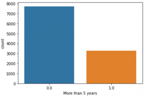
Figure 1. Biased data before over-sampling
Both classification and regression tasks are performed better by the proposed two-stage architecture than by the one-stage framework. The initial Linear-SVM and Logistic Regression classifiers outperformed the Naive Bayes classifier in terms of prediction accuracy during the classification stage. The improved random forests (RF) approach's second stage RMSE is less than that of the first-generation RF method and other feature selection methods. biased data before oversampling can be seen as in Figure 1.
4.3 Methodology
The majority of research on malignant growth projection is restricted to estimating how long a patient will live. The patient is then categorised as “made due” or “dead” after that. Due to the high mortality rate, the majority of people with hepatic malignant growth would be considered “dead”. How much longer these sufferers might have to put up with it is not yet known. The patient's likelihood of survival is predicted by a characterization model in the following section, and the patient's additional life expectancy is predicted by a relapse model for patients whose anticipated result is “dead.” With the exception of the fundamental AI categories, the two phases use the same strategies. To predict the endurance condition during the grouping step, three different classifiers are used: straight SVM classifiers, Naive Bayes classifiers, and RF classifiers. Regression models are used to project endurance months during the relapse period. There are two concerns that arise during the ordering process. The main problem is that a one-sided classifier would result from a one-sided preparation set. Cases from the minority class would be incorrectly categorised as being a part of the larger group. Information needs to be modified in order to address this problem. The quantity of the element pool and the poor quality of the characterization are the following problems. A selection of pool highlights is subjected to CHI2 Feature Selection using the fountain by a support vector machine classifier and a Nave Bayes classifier. During grouping execution, the flowing framework did not favor the initial classifier.
The phases of the classification framework are as follows:
1. Consulting the SEER database for statistics on MPCs such liver, lung, stomach, thyroid, and skin malignancies.
2. You can combine the data and rearrange them.
3. Separate the data into sets for training and testing.
4. To balance the dataset, employ SMOTE (Synthetic Minority Oversampling Technique).
5. Select the top characteristics for modelling using CHI2 Feature Selection.
6. Use the linear-SVM, Naive Bayes, and Logistic Regression classifiers for prediction.
7. Evaluate the outcomes that were predicted using error metrics like accuracy and f-score. The steps in the regression framework are as follows:
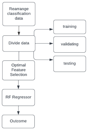
Figure 2. Methodology
The classifiers used in the classification were Linear SVM and Naive Bayes. It first creates a separating hyper plane between two classes before classifying samples according to distance. The data has been one-hot encoded using only zeros and ones as shown in Figure 2.
One-hot encoded data could be separated as needed using linear SVM and naive bayes. It used a series of random under sampling and CHI2 feature selection. The RF repressor was used throughout the regression step.
It was cascaded using feature selection depending on contribution score, just like a standard bagging Regressor [33-34].
4.4 Materials and methods
The free and open-source database SEER contains deidentified, organized, and annotated information regarding malignancies in the United States. The database is vast enough to offer many samples for machine learning algorithms to study. A qualified medical professional carried out the clinical or microscopic confirmation of a cancer diagnosis in the SEER cancer registries.
Most cancer prognosis studies merely predict the patient's life expectancy. The patient is then classified as either having “survived” or “died.” The majority of liver cancer patients would be considered “dead” because of the disease's high mortality rate. How long these patients will live is unknown. Therefore, we suggest a two-stage categorization strategy. A regression model is used to forecast the life expectancy of patients whose predicted outcome is “dead,” and a classification model is used to determine the patient's chance of surviving.
With the exception of the basic machine learning categories, both phases use the same approaches. In the classification stage, linear-SVM, Naive Bayes, and logistic regression classifiers are used to forecast the survival condition. In the regression stage, RF regressor and Decision Tree Regressor are used to estimate the survival months. The classification stage brings about two issues. The first problem is that the biassed training set would produce a biassed classifier. Minority-related cases would be wrongly categorised as falling under the purview of the majority group. To address this issue, data balance is required. The second problem, which has a negative impact on the classification outcome, is the size of the feature pool.
A support vector machine classifier and a Nave Bayes classifier are used in cascade with CHI2 Feature Selection to select a subset of features from the pool. When it comes to classification, the cascaded system outperforms the first classifier.
4.4.1 Algorithms applied
The classifiers utilised in the classification were Naive Bayes and linear SVM. It first creates a separation hyper plane between two classes, then sorts samples based on how far apart they are. The data, which is made up entirely of zeros and ones, was produced using one-hot encoding.
Using linear SVM and the Naive Bayes classifier, the demand for separating one-hot encoded data was satisfied. It cascaded with the selection of CHI2 characteristics. In the regression step, RF acted as the Regressor. As with a standard bagging Regressor, it was cascaded with contribution score-based feature selection.
4.4.2 Linear SVM
A dataset is said to be linearly separable when it can be separated into two classes by a single straight line, and the Linear SVM classifier is used to divide the dataset into its two groups. We use several machine learning approaches to forecast and categories data, depending on the dataset. The Support Vector Machine (SVM) is a linear model that can be used to solve classification and regression problems. It can be used in both linear and nonlinear circumstances and has a variety of practical applications. SVM operates on a straightforward principle: The algorithm draws a line or a hyper plane to categories the data. SVMs first locate the line (or hyper plane) separating the data into two classes. The SVM algorithm takes data as input and produces, if it is possible, a line that divides those classes.
4.4.3 Naïve Bayes
“Naive Bayes classifiers” refer to a group of classification techniques based on Bayes' Theorem. It is a collection of algorithms built on the premise that every pair of traits used to categorize anything stands alone from the other. Naive Bayes algorithms are extensively used in applications including sentiment analysis, spam filtering, recommendation systems, and others. Their main drawback is the need for independent predictors, despite the fact that they are quick and simple to deploy. In real-world situations, the predictors are frequently reliant, which reduces the classifier's efficacy. The Naive Bayes algorithm uses the Bayes theorem to solve classification problems in supervised learning. It is mostly utilised for text categorization and has a huge training dataset. Machine learning models that can learn fast and predict outcomes can be produced with the use of the Naive Bayes Classifier, a quick and effective classification algorithm. It provides predictions based on the likelihood of an item because it is a probabilistic classifier. Spam filtration, sentiment analysis, and article categorization are a few examples of common Naive Bayes Algorithm applications.
4.4.4 Random Forest
Random Forest is a well-known machine learning technique from the supervised learning paradigm. Artificial intelligence problems involving categorization and regression may be resolved with it. Its foundation is the principle of ensemble learning, a technique that combines a number of classifiers to address a challenging issue and improve model performance. The Random Forest classifier uses a number of decision trees on different subsets of the provided dataset. The average is used to increase the forecasting accuracy of the dataset, as the name suggests. The random forest employs the projections from each decision tree instead of just one to estimate the ultimate result based on the majority vote of predictions. The accuracy and likelihood of overfitting increase with the number of trees in the forest. Variance, one of Decision Trees' biggest weaknesses, is addressed with the machine learning technique Random Forests.
Decision Despite being flexible and simple, trees are a greedy algorithm. It focuses on optimizing for the current node split rather than how that split affects the entire tree. A greedy approach speeds up Decision but leaves them open to over fitting. An overfit tree that is highly optimized at predicting the values in the training dataset results in a high-variance learning model.
4.4.5 Logistic regression
When the outcome is binary, we use the logistic regression statistical modelling technique. Whether the independent variables are continuous or categorical, logistic regression modeling can be utilised to predict the outcome when the outcome variable is binary. The process of determining the probability of a discrete result from an input variable is known as logistic regression. A binary result, which can be true or false, yes or no, or another value, is a common characteristic in logistic regression models. Multinomial logistic regression can be used to model situations with more than two discrete outcomes. Logistic regression is a useful analysis method that may be used to identify whether a fresh sample belongs in a given category. due to various reasons Analytical techniques like logistic regression are useful for classifying cyber security problems like attack detection. For problems involving binary and linear classification, logistic regression is a simpler and more efficient approach. It is an easy-to-use classification model with linearly separable classes that delivers excellent outcomes. It is a classification technique that businesses regularly use. Similar to the Adaline and Perceptron, the logistic regression model is a statistical method for binary classification that can be expanded to multiclass classification. Scikit-highly learn's efficient logistic regression implementation is capable of handling multiclass classification workloads.
4.4.6 Decision tree
The decision tree method is one of the supervised machine learning techniques. It can be used to solve classification and regression issues. This approach aims to build a model that forecasts the value of a target variable. To do this, a decision tree is utilised, which visualizes the problem as a tree with features expressed on the core node and a leaf node corresponding to a class label. The decision tree algorithm is a member of the supervised learning algorithm family. The decision tree approach can be utilised to address classification and regression problems, unlike other supervised learning methods.
The goal of using a decision tree is to create a training model that can predict the type or value of a target variable and learn fundamental decision rules from previous data (training data). We forecast the class label of a record in decision trees by starting at the root of the tree. We compare the values of the record attribute to those of the root attribute. By following the branch that leads to that value's value in light of the comparison, we go on to the subsequent node. The selection of important splits has a significant impact on how accurate a tree is. Regression and classification trees have different selection criteria. To decide whether to split a node into sub nodes, decision trees use a variety of procedures. The expansion of sub-nodes increases the homogeneity of the next sub-nodes. The purity of the node increases with respect to the target variable. The decision tree divides the nodes into groups based on all of the available attributes before choosing the grouping that produces the most homogeneous sub-nodes.
4.4.7 Oversampling and under sampling
A considerable skew in the class distribution can be detected in unbalanced datasets, such as 1:100 or 1:1000 samples in the minority class relative to the majority class. Many machine learning algorithms may be impacted by this bias in the training dataset, while others may totally ignore the minority class. Since minority projections could possibly be the most crucial, this is an issue. Resampling the training dataset at random is one method for addressing class imbalance. The two main methods for randomly resampling an unbalanced dataset are under sampling, or eliminating samples from the majority class, and oversampling, or including examples from the minority class.
Oversampling and under sampling for unfair categorization are the two main strategies for random resampling.
Duplicate samples drawn at random from the minority class by oversampling.
Random Remove instances from the majority class at random when sampling.
The practice of randomly picking instances from the minority class and replacing them in the training dataset is known as random oversampling. The act of randomly picking instances from the majority class and eliminating them from the training dataset is known as random under sampling. Both methods can be used repeatedly up until the training dataset achieves the desired class distribution, such as an equal split across the classes.
Since they don't use heuristics or make assumptions about the data, these techniques are referred to as “naive resampling” methods. They are therefore easy to use and quick to complete. For extremely large and complex datasets, it works perfectly. Both approaches can be used to categories problems into groups of two (binary) or many groups, each of which may include one or more majority or minority classes. Importantly, the class distribution adjustment is only applied to the training dataset. The goal is to modify the models' fit. The test or holdout datasets used to evaluate a model's performance don't need to be resampled. The specifics of the dataset and models being utilised also play a role in whether these crude strategies are effective in general. Duplicate samples from minority classes are included in the training dataset as part of the random oversampling technique. This approach may be advantageous for machine learning algorithms that are affected by skewed distributions and when multiple variables are present. Duplicate examples for a certain class may have an impact on model fit. It may be necessary to use iterative learning coefficients-based techniques, including stochastic gradient descent-based artificial neural networks. Support vector machines and decision trees are two models that could be affected.
4.5 Chi square feature selection
The act of eliminating the most crucial features from a dataset and then utilizing machine learning methods to enhance the performance of the model is referred to as feature selection, also known as attribute selection. The chance of over fitting increases and training time is greatly increased by a large number of useless characteristics.
4.5.1 Chi-square feature extraction
Use the Chi-square test to draw categorical characteristics from a dataset. The features with the greatest Chi-square scores are picked after the Chi-square test is run between each feature and the target. It establishes if the sample's representation of the relationship between two category variables accurately captures that relationship in the population.
The Chi-Square feature selection method is a popular method for selecting features from text data. In statistics, the 2 test is used to prove the independence of two events. Ascertain whether the choice of features is independent of the occurrence of a certain term and a corresponding class.
$X^2=\frac{({ Observed\,\, frequency }- { Expected\,\, frequency })^2}{{ Expected\,\, frequency }}$
The Chi-Square test is used to assess how comparable the relative variances of two distributions are. The assumption underlying its null hypothesis is that the supplied distributions are independent. Thus, this test may be used to determine the best features for a given dataset by determining which characteristics depend on the output class label the most. The CHI2 value for each feature in the dataset is calculated, and the features are then sorted using the CHI2 value in decreasing order. The higher the CHI2 values, the more the output label depends on the feature and the more important the feature is in defining the output. The Chi-Square test's application in machine learning and its outcomes are hotly contested topics. Since we will have a number of features in line and must choose the best ones to build the model, feature selection is a significant challenge in machine learning. By looking at how the attributes are related to one another, the chi-square test assists in feature selection.
In statistics, the chi-square test is used to determine if two events are unrelated to one another. We can determine the observed count O and the expected count E from the data of two variables. The Chi-Square formula is used to determine the difference between the observed count O and the anticipated count E.
When two features are independent, the observed count is fairly close to the anticipated count; as a result, the Chi-Square value is smaller. anticipated amount In the event when the Chi-Square value is large, the independence hypothesis is false. Simply said, the higher the Chi-Square value and better it is for model training, the more dependent a feature is on the response.
4.5.2 Limitations
Chi-Square is sensitive to low frequencies in table cells. In general, chi-square can yield inaccurate results if a table cell's predicted value is less than 5.
Imbalanced data is a common problem in machine learning, which brings challenges to feature correlation, class separation and evaluation, and results in poor model performance. A classification data set with skewed class proportions is called imbalanced. Classes that make up a large proportion of the data set are called majority classes. Those that make up a smaller proportion are minority classes.
The improvement of the classification stage consists of CHI2 feature selection and SMOTE (Synthetic Minority Oversampling Technique) oversampling. The table below lists the classification performance measures for SVC, Gaussian Nave Bayes, and Logistic Regression. The performance criteria utilised for comparison include the F1 score, accuracy, and confusion matrix. Regression performance metrics include the R2 score, RMSE, and MAE.
5.1 Classification stage
We had used label encoding to convert text input into numerical data. The sections above have discussed the subject of the class gap. As can be seen in Figure 2, the “less than 5 years of survival” class of cases outnumbers the other class of cases. Over-sampling is one of the most widely used methods for addressing the problem of class inequality. We had considered the SMOTE oversampling method in this instance due to the tiny size of the dataset. After SMOTE was used, the dataset's size grew from 10985 to 15439 cases.
Out of a total of 16 characteristics, we have selected the best six features using CHI2-based feature selection. The CHI2-feature selection determined the following six features to be the top ones:
One to three groups of data were selected. The data contained 3860 train cases and 11,759 test cases, respectively. The classifiers assigned labels of 0 and 1, respectively, for patients whose projected survival time is less than 60 months and for patients whose expected survival time is more than five years. The SVC has the greatest F1 score of the three models, at 0.788, and is also the most accurate.
The accuracy and F1 score of the three models are presented below the table along with the Confusion matrix's findings as shown in Figure 3, Table 1 and Table 2 are the clear evident of the achieved results.
Figure 3. Classification stage
Results after applying SMOTE: 0-cases with less than 5 years of survival, 1-cases with more than 5 years of survival.
Table 1. Accuracy and F1 score of the three classification models
|
MODEL |
ACCURACY |
F1 SCORE |
|
Gaussian Naïve Bayes |
74.63 |
0.769 |
|
Logistic Regression |
77.74 |
0.763 |
|
Support Vector Classifier |
78.54 |
0.788 |
Table 2. Results from the confusion matrices of the three classification models
|
MODEL |
PREDICTED 0 |
PREDICTED 1 |
ACTUAL |
|
Gaussian Naïve Bayes |
1251 |
728 |
0 |
|
251 |
1630 |
1 |
|
|
Logistic Regression |
1613 |
366 |
0 |
|
493 |
1388 |
1 |
|
|
Support Vector Classifier |
1488 |
491 |
0 |
|
337 |
1544 |
1 |
|
| MODEL | R2 SCORE | RMSE | MAE |
| Random Forest Regressor | 0.42 | 32.03 | 21.60 |
| Decision Tree Regressor | 0.41 | 32.29 | 21.69 |
5.2 Regression stage
The output of the classification stage was filtered to only contain cases with predicted labels of 0. (less than five years of survival time). Regression models based on decision trees and random forests are utilised. The comparative metrics for these two models are R2, RMSE, and MASE. The Models random forest regressor is the more robust of the two, with the lowest RMSE and MAE.
Most contemporary survival analyses focus on the connections between patient variables and likelihood of five-year survival. Most of the answers to the specific topic of how long a patient with concurrent cancer will live are still unknown. The patient-specific survival time of cancer patients with coexisting diseases was projected in this experiment. It divides the specific query into two machine learning problems. The first issue is the separation between patients who will live more than five years and those who won't. The second phase entails creating a regression model that predicts the patient's likelihood of surviving for five years.
Among the most common cancers are those of the lung, liver, stomach, thyroid, and skin. Predicting the prognosis of cancer patients can be helpful for medical professionals, patients, and families. The suggested two-stage method forecasts a patient's survival as well as how many months they will live. Whether a patient will live for more than five years is predicted in the first stage. If the forecast is death, the second stage calculates the patient's remaining months of life. In the classification phase during feature selection, scaling of features is used. During the regression stage, the Random Forest Classifier is utilised.
Accuracy can be improved even more by using feature selection during the regression phase. The feature selection process can be improved by looking into interdisciplinary and intradisciplinary dispersions. In the future, we'll continue to investigate feature selection strategies that could improve our current prediction performance. Another MPC that may be researched is second primary breast cancers.
[1] Howlader, N., Noone, A.M., Krapcho, M., et al. (2019). SEER cancer statistics review, 1975-2016, National Cancer Institute. Bethesda, MD. https://seer.cancer.gov/archive/csr/1975_2016/#contents.
[2] Curtis, R.E. (2006). New Malignancies Among Cancer Survivors: SEER Cancer Registries, 1973-2000. US Department of Health and Human Services, National Institutes of Health, National Cancer Institute.
[3] Diederichs, C., Berger, K., Bartels, D.B. (2011). The measurement of multiple chronic diseases-A systematic review on existing multimorbidity indices. Journals of Gerontology Series A: Biomedical Sciences and Medical Sciences, 66(3): 301-311. https://doi.org/10.1093/gerona/glq208
[4] Edwards, B.K., Noone, A.M., Mariotto, A.B., et al. (2014). Annual report to the nation on the status of cancer, 1975-2010, featuring prevalence of comorbidity and impact on survival among persons with lung, colorectal, breast, or prostate cancer. Cancer, 120(9): 1290-1314. https://doi.org/10.1002/cncr.28509
[5] Zolbanin, H.M., Delen, D., Zadeh, A.H. (2015). Predicting overall survivability in comorbidity of cancers: A data mining approach. Decision Support Systems, 74: 150-161. https://doi.org/10.1016/j.dss.2015.04.003
[6] Wang, Y., Wang, D., Ye, X., Wang, Y., Yin, Y., Jin, Y. (2019). A tree ensemble-based two-stage model for advanced-stage colorectal cancer survival prediction. Information Sciences, 474: 106-124. https://doi.org/10.1016/j.ins.2018.09.046
[7] Lynch, C.M., Abdollahi, B., Fuqua, J.D., de Carlo, A.R., Bartholomai, J.A., Balgemann, R.N., van Berkel, V. H., Frieboes, H.B. (2017). Prediction of lung cancer patient survival via supervised machine learning classification techniques. International Journal of Medical Informatics, 108: 1-8. https://doi.org/10.1016/j.ijmedinf.2017.09.013
[8] NCI SEER Overview. (2015). Overview of the Seer Program. Surveillance Epidemiology and end Results. http://seer.cancer. gov/about/, accessed on Dec. 10, 2023.
[9] Liu, P., Li, L., Yu, C., Fei, S. (2020). Two staged prediction of gastric cancer patient’s survival via machine learning techniques. In Proceedings of the 7th International Conference on Artificial Intelligence Applications, 105-116. https://doi.org/10.5121/csit.2020.100308.
[10] Garzín, B., Emblem, K.E., Mouridsen, K., et al. (2011). Multiparametric analysis of magnetic resonance images for glioma grading and patient survival time prediction. Acta Radiologica, 52(9): 1052-1060. https://doi.org/10.1258/AR.2011.100510
[11] Magome, T., Haga, A., Igaki, H., et al. (2014). TH-E-BRF-05: comparison of survival-time prediction models after radiotherapy for high-grade glioma patients based on clinical and DVH features. Medical Physics, 41(6Part33): 570-570. https://doi.org/10.1118/1.4889669
[12] Roffo, G., Melzi, S., Castellani, U., Vinciarelli, A. (2017). Infinite latent feature selection: A probabilistic latent graph-based ranking approach. In Proceedings of the IEEE International Conference on Computer Vision, Venice, Italy, pp. 1398-1406. https://doi.org/10.48550/arXiv.1707.07538
[13] Roffo, G. (2020). Feature Selection Library, MATLAB Central File Exchange. https://in.mathworks.com/matlabcentral/fileexchange/56937-feature-selection-library, accessed on Dec. 12, 2023.
[14] Li, Z., Yang, Y., Liu, J., Zhou, X., Lu, H. (2012). Unsupervised feature selection using nonnegative spectral analysis. In Proceedings of the AAAI Conference on Artificial Intelligence, 26(1): 1026-1032. https://doi.org/10.1609/aaai.v26i1.8289
[15] Yang, Y., Shen, H.T., Ma, Z., Huang, Z., Zhou, X. (2011). ℓ2, 1-norm regularized discriminative feature selection for unsupervised learning. In IJCAI International Joint Conference on Artificial Intelligence, 1589-1594. http://hdl.handle.net/10453/119490.
[16] Li, J., Cheng, K., Wang, S., Morstatter, F., Trevino, R.P., Tang, J., Liu, H. (2017). Feature selection: A data perspective. ACM computing surveys (CSUR), 50(6): 1-45. https://doi.org/10.1145/3136625
[17] Song, F., Guo, Z., Mei, D. (2010). Feature selection using principal component analysis. In 2010 international conference on system science, engineering design and manufacturing informatization, Yichang, China, pp. 27-30. https://doi.org/10.1109/ICSEM.2010.14
[18] Liu, Y.Q., Wang, C., Zhang, L. (2009). Decision tree based predictive models for breast cancer survivability on imbalanced data. In 2009 3rd International Conference on Bioinformatics and Biomedical Engineering, Beijing, China, pp. 1-4. https://doi.org/10.1109/ICBBE.2009.5162571
[19] Thongkam, J., Xu, G., Zhang, Y., Huang, F. (2008). Breast cancer survivability via AdaBoost algorithms. In Proceedings of the second Australasian workshop on Health data and knowledge management, 80: 55-64. https://vuir.vu.edu.au/id/eprint/5293., accessed on Dec. 12, 2023.
[20] Park, K., Ali, A., Kim, D., An, Y., Kim, M., Shin, H. (2013). Robust predictive model for evaluating breast cancer survivability. Engineering Applications of Artificial Intelligence, 26(9): 2194-2205. https://doi.org/10.1016/j.engappai.2013.06.013
[21] Kaviarasi, R., Gandhi, R.R. (2019). Accuracy enhanced lung cancer prognosis for improving patient survivability using proposed Gaussian classifier system. Journal of Medical Systems, 43(7): 1-9. https://doi.org/10.1007/s10916-019-1297-2
[22] Liu, H., Su, Z., Liu, S. (2013). Improved CHI text feature selection based on word frequency information. Computer Engineering and Applications, 49(22): 110-114.
[23] Ryu, S.M., Lee, S.H., Kim, E.S., Eoh, W. (2019). Predicting survival of patients with spinal ependymoma using machine learning algorithms with the SEER database. World Neurosurgery, 124: e331-e339. https://doi.org/10.1016/j.wneu.2018.12.091
[24] Kleinlein, R., Riaño, D. (2019). Persistence of data-driven knowledge to predict breast cancer survival. International Journal of Medical Informatics, 129: 303-311. https://doi.org/10.1016/j.ijmedinf.2019.06.018
[25] Naghizadeh, M., Habibi, N. (2019). A model to predict the survivability of cancer comorbidity through ensemble learning approach. Expert Systems, 36(3): e12392. https://doi.org/10.1111/exsy.12392
[26] Donin, N.M., Kwan, L., Lenis, A.T., Drakaki, A., Chamie, K. (2019). Second primary lung cancer in United States cancer survivors, 1992-2008. Cancer Causes & Control, 30: 465-475. https://doi.org/10.1007/s10552-019-01161-7
[27] Adamo R.J.M., Dickie, L. (2018). SEER program coding and staging manual. In U.S. Department of Health and Human Services National Institutes of Health National Cancer Institute. Bethesda, MD, USA: National Cancer Institute.
[28] Roffo, G., Melzi, S., Cristani, M. (2015). Infinite feature selection. In Proceedings of the IEEE International Conference on Computer Vision, Santiago, Chile, pp. 4202-4210. https://doi.org/10.1109/ICCV.2015.478
[29] Japkowicz, N. (2000). The class imbalance problem: Significance and strategies. In Proceedings of the International Conference on Artificial Intelligence, 56: 111-117.
[30] Ali, L., Zhu, C., Golilarz, N.A., Javeed, A., Zhou, M., Liu, Y. (2019). Reliable Parkinson’s disease detection by analyzing handwritten drawings: construction of an unbiased cascaded learning system based on feature selection and adaptive boosting model. IEEE Access, 7: 116480-116489. https://doi.org/10.1109/ACCESS.2019.2932037
[31] Roffo, G., Melzi, S. (2016). Features selection via eigenvector centrality. Proceedings of new frontiers in mining complex patterns (NFMCP 2016), 1-12.
[32] Peng, H., Long, F., Ding, C. (2005). Feature selection based on mutual information criteria of max-dependency, max-relevance, and min-redundancy. IEEE Transactions on Pattern Analysis and Machine Intelligence, 27(8): 1226-1238. https://doi.org/10.1109/TPAMI.2005.159