Selvaraj Karupusamy | Sundaram Maruthachalam | Suresh Mayilswamy | Shubham Sharma | Jujhar Singh | Giulio Lorenzini*
© 2021 IIETA. This article is published by IIETA and is licensed under the CC BY 4.0 license (http://creativecommons.org/licenses/by/4.0/).
OPEN ACCESS
Numerous challenges are usually faced during the design and development of an autonomous mobile robot. Path planning and navigation are two significant areas in the control of autonomous mobile robots. The computation of odometry plays a major role in developing navigation systems. This research aims to develop an effective method for the computation of odometry using low-cost sensors, in the differential drive mobile robot. The controller acquires the localization of the robot and guides the path to reach the required target position using the calculated odometry and its created new two-dimensional mapping. The proposed method enables the determination of the global position of the robot through odometry calibration within the indoor and outdoor environment using Graphical Simulation software.
odometry, navigation, mapping, localization, range finders, simulation
Autonomous mobile robots are required for supporting humans in nonliving areas such as underwater and space research. They are useful for research activities such as monitoring, cleaning, searching, and inspection. The mobile robots stand for the evolution of these as they can move freely in a dynamic environment. The propagation of mobile robots is subjected to handling two major problems, which are:
The proposed method is used to enhance the capability of localization, which depends on odometry and improves the navigation system. This makes the path planning to become more flexible and easily pertinent. To deal with the localization problem, first, we need to apply an odometry calibration method. To that method, we need to integrate odometry errors right through a path traveled by the robot and bring into new improved odometry parameters. This method is an endpoint method with diverse initial and final points, which do not require additional sensors. Robots sense and transfer the information to the remote station by wireless communication systems. An important advantage of the method is that it is compatible with any odometry model.
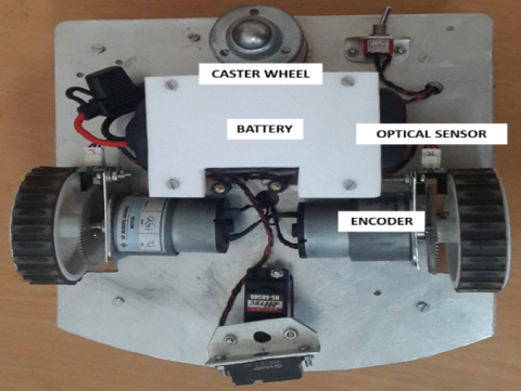
In this work, the development of a differential drive mobile robot for autonomous navigation system is described. Figure 1(a) shows the top view of the differential drive mobile robot and Figure 1(b) shows the bottom view of the differential drive mobile robot.
The global position of the robot is mapped using the odometry data from the robot encoders and the robot can effectively avoid obstacles. Local reconstruction of the robot’s position and orientation is made possible with an accurate odometry calibration from the encoder’s data [1]. The infrared (IR) range finder is a low-cost, lightweight, and low-power-consumption device compared to a laser range finder for an indoor environment. It deals with two-dimensional (2D) mapping and localization. This is built by a 2D grid map in local coordinate, using data from the IR range finder. It is integrated into the global coordinate of a mobile robot using information from IR landmarks. A Wi-Fi (wireless networking) transmitter is used to transmit the odometry and local reconstruction information. It provides a consistent global map that can be used in the autonomous navigation of mobile robots in remote locations [2, 3]. The experimental result under indoor environment is obtained by Virtual Simulation software.
(a)
(b)
Figure 1. Differential drive mobile robot: (a). Top view; (b) Bottom view
The designed differential drive robot has several components, including controller, sensors, motors, and actuators. The controller is the brain of the robot that helps to acquire the values from the sensors. and transmits the acquired values to a remote station through Wi-Fi. The architecture of the differential drive mobile robot is shown in Figure 2. In the environment, the developed algorithm plots a 2D map of the path traveled by the robot based on the collected information. The designed robot has two types of sensors to identify the environmental state. The first one is for finding the distance of the obstacle placed in front of the robot. Another one is to estimate the robot position. The robot algorithm has been simultaneously computing the sensors data as localization and mapping [1, 4 ,5]. The current position (x, y, ɵ) value will displayed through the LCD (liquid crystal display) that is placed on the robot itself. A sequential flowchart for system design is shown in Figure 3.
Figure 2. The architecture of the differential drive mobile robot
Figure 3. Sequential flowchart for system design
3.1 Differential drive wheel
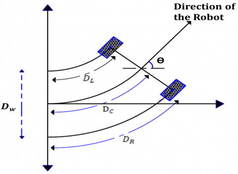
The two-wheeled differential drive robot is driven by two independently operated wheels placed on both sides of the robot body. The robot will go in a straight line when both the wheels are driven in the same direction and speed. When both wheels are turned with equal speed in opposite directions, the robot will rotate on the central point of the axis [6]. Figure 4 shows the direction of the robot when moving towards left direction. As the direction of the robot depends on the direction of rotation of the two driven wheels, this quantity of encoder pulse should be sensed and controlled precisely [3, 7].
Figure 4. Differential drive wheel position
where, $D_{\mathrm{W}}$ is the distance between the two wheels (mm).
The robot was driven on a surface of 5 m × 7.5 m in an indoor environment. A consistently smooth cement concrete floor was used as the landscape that normally reduced the chance of nonsystematic errors such as wheel slippage. The overall weight of the robot was 1.5 kg and the distance between the two wheels was 180 mm. The maximum speed was up to 300 mm/s. Encoders were used to calculate the linear displacement of each wheel. The new orientation of the robot could be estimated from the difference in the encoder counts, the diameter of the wheels, and distance between the wheels [1-5, 8-13]. The encoder values were transferred to the remote station system through the wireless data transmission module to plot a 2D map in the Virtual Simulation software.
3.2 Odometry computation method
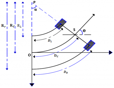
The odometry uses the data from motion sensors, to approximate the changes in the position relative to the starting point of the robot over time. This computation method calculates the position of the robot (X, Y, Ө) (X and Y are the coordinates of the ground plane and Ө is the direction of the robot). As this method is implemented in the differential drive mobile robot, the mapping calculation according to its movement is quite complex. The proposed method is used to simplify the complexity of the existing method by acquiring the current position of both (right and left) wheels in graphical display at every millisecond. In that way, the Simulation software algorithm can monitor the updated values of (x, y, Ө) at a time; ‘t’ is updated with the previous positional value (x, y, Ө). The displacement of the robot is based on its size and it is calculated by d = 2πr, where r is the radius of the wheel. Analysis of the robot motion is shown in Figure 5. Let the starting point of the robot be zero. In this method, the developed algorithm calculates the displacement of the wheel using pulses obtained from the encoders, placed in the wheel [3]. Let the number of counting pulses be n, then the wheel displacement is given by,
$d=\frac{n 2 \pi r}{\text { Total number of pulses per one revolution }}$ (1)
d – wheel displacement (mm)
r – radius of the wheel (mm)
n – counted pulse
Figure 5. Differential drive robot moving from the starting point
The robot covers distances at a time t. The arc length distance from the center point is Dc, which is calculated from the below equation,
$D_{\mathrm{C}}=\frac{D_{\mathrm{L}}+D_{\mathrm{R}}}{2}$ (2)
$D_{\mathrm{L}}$ – travel distance of the left wheel (in mm)
$D_{\mathrm{R}}$ – travel distance of the right wheel (in mm)
The direction of the robot depends on $\theta$ degree, to be rotated. The moving distance of the left wheel is less than that of the right wheel. So, the robot moves toward the left side or the first quadrant. The arc length of each wheel is different in radius but common concerning the center point, by considering wheel radius as $\mathrm{L}_{r} \text { and } \mathrm{R}_{r}$. Figures 5 and 6 show the representation of the wheel movement. These values are calculated from the basic geometry functions. The angles and $\theta$ are equal.
$\alpha=\frac{D_{\mathrm{L}}-D_{\mathrm{R}}}{D_{\mathrm{w}}}$ (3)
α is the angle difference in radians from the starting point, as shown in Figure 5.
where,
$R_{\mathrm{L}}=\frac{D_{\mathrm{L}}}{\alpha}$ (4)
From Eq. (4),
$\alpha R_{\mathrm{L}}=D_{\mathrm{L}}$ (5)
$R_{\mathrm{r}}=\frac{D_{\mathrm{R}}}{\alpha}$ (6)
From Eq. (6),
$\alpha R_{\mathrm{r}}=D_{\mathrm{R}}$ (7)
$\frac{\left(\mathrm{R}_{\mathrm{L}}+\mathrm{R}_{\mathrm{r}}\right)}{2}=R_{\mathrm{C}}$ (8)
$R_{\mathrm{C}}$ is the radius of the center point of the robot wheels.
From Eqns. (5) and (7),
$\begin{aligned}
&\alpha R_{\mathrm{L}}+\alpha R_{\mathrm{r}}=D_{\mathrm{L}}+D_{\mathrm{R}} \\
&\alpha\left(R_{\mathrm{L}}+R_{\mathrm{r}}\right)=D_{\mathrm{L}}+D_{\mathrm{R}}
\end{aligned}$ (9)
From Eq. (8),
$\left(R_{\mathrm{L}}+R_{\mathrm{r}}\right)=2 R_{\mathrm{C}}$ (10)
Substituting (10) in (9),
$2 \alpha R_{\mathrm{C}}=\mathrm{D}_{\mathrm{L}}+\mathrm{D}_{\mathrm{R}}$ (11)
$R_{\mathrm{C}}=\frac{D_{\mathrm{L}}+D_{\mathrm{R}}}{2 \alpha}$ (12)
Let the starting positions of the robot be X and Y, and they are denoted by equations as
$X=x+R_{\mathrm{C}} \cos \theta$ (13)
$Y=y+R_{\mathrm{C}} \sin \theta$ (14)
X, Y, $\theta$ are current positions of the robot at every millisecond. $\mathrm{X}_{\text {new }}, Y_{\text {new, }}, \theta_{\text {new }}$ are global positions of the robot that can be calculated from these equations. This is a continuous process during the entire task. So, the computation of the new position and the current robot position is done [13]. Figure 6 depicts the representation of position at each moment.
3.3 Navigation system
Let the starting position of the robot be S1, at the time t1 and let the next position be S2, at the time t2. At the time t1, the robot moves toward the left side. But the moving distance of the left wheel is found to be higher than that of the right wheel at time t2. So, the robot starts to move toward the right side from point S2. While the robot moves in the right side, the center point of the arc is placed on the right side, as shown in Figure 6.
$D_{\mathrm{L}}, D_{\mathrm{R}}, \text { and } D_{\mathrm{C}}$ are calculated from the robot wheel movements. This will be helpful to find the radius of the arc $R_{\mathrm{L}}, R_{\mathrm{C}} \text {, and } R_{\mathrm{r}}$ and thereby the new position of the robot $\left(X_{\text {new }}, Y_{\text {new }}, \theta_{\text {new }}\right)$ will be calculated. The latest position values are replaced with the previous position values and the software algorithm performs the calculation and updates the current path of the robot [9].
A new angle of the robot can be calculated using Eq. (10),
$\theta_{\mathrm{N}}=\alpha \times 180 / \pi$ (15)
Calculation of the actual position of the robot is given below:
$\begin{gathered}
X=\left[X_{\text {new }}\right]+R_{\mathrm{C}} \cos \left(\theta_{\mathrm{N}}+\theta\right) \\
X=\left[x+R_{\mathrm{C}} \cos \theta\right]+R_{\mathrm{C}} \cos \left(\theta_{\mathrm{N}}+\theta\right) \\
X=x+R_{\mathrm{C}}\left[\cos \theta+\cos \left(\theta_{\mathrm{N}}+\theta\right)\right] \\
Y=\left[Y_{\text {new }}\right]+R_{\mathrm{C}} \sin \left(\theta_{\mathrm{N}}+\theta\right)
\end{gathered}$ (16)
Figure 6. Odometry calculation of the robot at instant time
$\begin{gathered}
Y=\left[y+R_{\mathrm{C}} \sin \theta\right]+R_{\mathrm{C}} \sin \left(\theta_{\mathrm{N}}+\theta\right) \\
Y=y+R_{C}\left[\sin \theta+\sin \left(\theta_{\mathrm{N}}+\theta\right)\right]
\end{gathered}$ (17)
$\theta_{\text {new }}=\theta+\theta_{\mathrm{N}}$ (18)
The above is a simplified odometry function for differential drive mobile robot.
The differential drive robot performs autonomous movement by acquiring robot position and orientation with the help of accurate odometry calculation. The calculation is done from the starting position of the robot with the help of the encoder’s readings, from which the global position of the robot within the environment can be determined [14, 15].
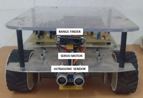
Figure 7. Differential drive mobile robot with an IR range finder and ultrasonic sensor
$\text { Distance }=\frac{\text { Speed of sound } \times \text { Time taken }}{2}$
Ultrasonic sensors can measure distance. The device emits an ultrasonic wave and receives the wave reflected from the object. Distance measurement can be achieved by measuring the time between the emission and reception. Here, the developed controller algorithm controls the movement of wheels. Time-calculated odometry values help in identifying the robot path and direction by integrating the value into the global coordinate of the mobile robot. The IR range finder works by the process of triangulation. Figure 7 shows that the experimental test is differential drive mobile robot with an IR range finder and ultrasonic sensor.
A pulse of light is emitted and then reflected back. When the light returns, it comes back at an angle that is dependent on the distance of the reflecting object. Triangulation works by detecting this reflected beam angle. By knowing the angle, distance can be determined [12].
4.1 Localization and mapping
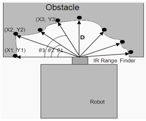
Robotic mapping is a field related to computer vision and capturing environmental data. The IR range finder is used to map the environment. The robot needs at least one range finder and one nonmodified servo. When the ultrasonic sensor detects any obstacle, the servo starts to rotate to a particular degree and record the coordinate values [2, 12]. Then again servo moves to the next available angle and notes the same.
The system performs the process of monitoring environment and collecting the point cloud data continuously. Figure 8 shows the servo mapping system (servo motor with IR range finder) can achieve in front of 180° rotation. It has an array of coordinates for the corresponding angle. After the first cycle, the servo system must rotate back in the reverse direction and record the values. This technique helps to perform the mapping process. The following figures shows that the experimental test is performed in a single room by placing some obstacles in different places [10].
Figure 8. Mapping with the IR range finder
When the robot is powered on in the indoor environment, the previously measured robot position and the global position are interconnected. The computed position is saved as a relative position. Robots’ movement toward the captured data and it will be compared with already saved mapped data for localization [16, 17].
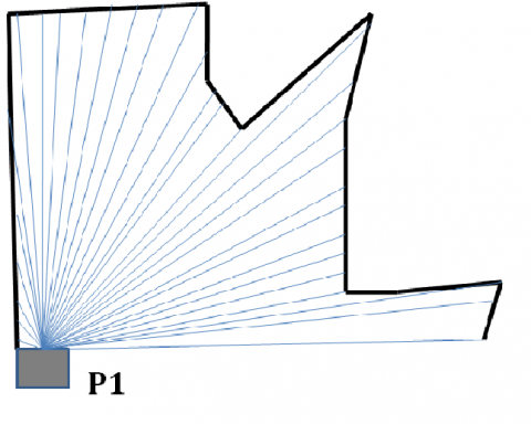
Figure 9. Scanning of objects at position P1
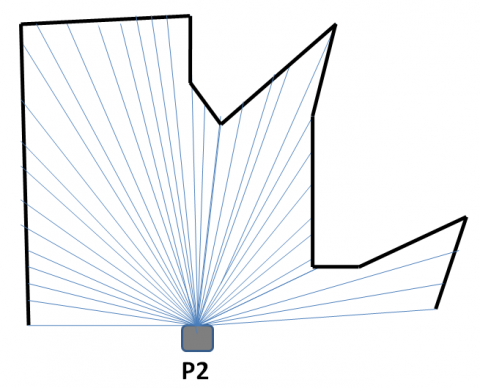
Figure 10. Scanning of objects at position P2
Figure 11. Mapped data at P1
Figure 12. Mapped data at P2
In case of its matching with the data in its localization position, the orientation of the robot position automatically gets data from the global position. Figures 9 and 10 show the robot position scanning of the room with two objects. Figures 11 and 12 show the structure of the scanning data at different positions of the robot. Finally, both mapped images are the same. This can be synchronized with the robot’s stored mapping data for localization process.
Localization is helpful for the robot to make a decision and achieve target position along with identifying the shortest path without human knowledge. The user can provide the whole environment structure to the robot. The constructed data can contain wall position, angles, clutter shape, and its position data [12, 18]. Every individual room structure can be saved in different segments. Low-resolution sensors can make more noise in this mapping structure. Noise is produced during comparison errors in the localization process. This can be reduced by the use of a noise-reducing algorithm in the localization of clutter.
4.2 Experiment in an indoor environment
The robot starts to move from the home position autonomously and also navigates the path to avoid the obstacle in the room. At the same time, the main controller simultaneously calculates the robot position (x, y, $\theta$) and displays the same in LCD, and in addition, transmit it to the computer in the remote location [19]. The simulation program starts to plot the values as a 2D graph to trace the robot path [20]. The robot starting position is considered as the origin of the plotting graph. The robot scanning process starts when it meets an obstacle in the moving path. Otherwise, it will be moving toward the target. These works enable to study and analyze the errors of the odometry computation and thereby calculate its efficiency. Figure 13 shows the robot’s moving direction while avoiding the obstacle in its path.
Figure 13. Robot moving path with indoor structure
4.3 Efficient odometry computation
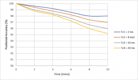
The experimental test is conducted at a different speed, different cyclic time for calculation in a room. In this test, an examination regarding the difficulties in finding the exact position and path of the robot is performed. Figure 14 represents the accuracy of function concerning time. Computation speed and accuracy are depending on the number of mathematical functions in the algorithm. In this odometry, only the minimum number of multiplication and additions are used. This algorithm does not have integral, differentiation, and matrix functions. So, it takes the least time for the computing process. Other major odometry parameters are given below.
4.3.1 Wheel friction
Friction of the wheel affects the position accuracy. Sometimes the rotation of wheels could slip by the smooth surface. But the encoder gives out pulses while the robot not moving. This may give out wrong positional value during the odometry. This problem can be avoided by using high friction tires or using wheels with better width.
4.3.2 Computing speed
Computation of the odometry should take maximum slot time. When time increases, the difference between every computation is ignored; thereby, the positional changes get differed. These mainly affect the calculation of direction changes.
4.3.3 Number of pulses per revolution
Encoder output is directly related to the accuracy. The number of pulses is directly proportional to the resolution.
4.3.4 Distance between the two wheels.
Distance between the two wheels is directly proportional to the accuracy. This parameter can efficiently measure minimum level turning difference.
4.3.5 Diameter of the wheel
Positional accuracy depends on the diameter of the wheel. Its accuracy is inversely proportional to the size of the wheel.
This work explained the experimental result of the robot motion computing speed and accuracy in odometry computation. The graph is floating between the robot motion time increments and the accuracy level of the position computation. The accuracy level percentage can be calculated from the traveled distance and deviation of the actual position at unit time.
$\begin{gathered}
\text { Position Accuracy } \\
=\frac{\text { Displaced position - Target position }}{\text { Total Displacement }} \times 100 \%
\end{gathered}$
This experiment can check the accuracy level at different computation speeds. Figure 14 shows various levels of accuracy explaining different computation periods.
Figure 14. Experimental graph plotted for various computing speeds
4.4 Odometry experimental analysis
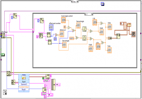
Figure 15. Block diagram for plotting a robot path on a virtual screen
The computation of the robot is at maximum accuracy at the starting point. The position of the robot at the starting point is accurate and it is calculated from that point [21]. But the position accuracy gets degraded when the time and position increase. So, the position error is rapidly increased. The maximum error occurs when the direction of the robot gets changed. Robot position accuracy variation is calculated for every period. The position accuracy can be calculated as,
$Odometry position accuray
=\frac{\text { Robot actual position sination point }}{\text { Tobot traveling distance }}
$
Traveling distance Ds = $D_{\mathrm{s}}=\sqrt{\left(x_{t}-x_{\text {start }}\right)^{2}+\left(y_{t}-y_{\text {start }}\right)^{2}}$
$x_{t}$ is the robot displacement on x-axis at time t.
$\chi_{\text {start }}$ is the starting position of the robot on x-axis.
$y_{t}$ is the robot displacement on y-axis at time t.
$y_{\text {start }}$ is the starting position of the robot on y-axis.
Calculated position data can be wirelessly sent to the remote station and it has several modules that segment the received data from the robot. The remote station monitoring system has virtual simulation software that can process the position and mapped data. Figure 15 shows the block diagrams of the software programming for calculating the robot path. This computation method is very useful for error analysis, which is done by calibration.
On the basis of the signal arriving from robots and it will be chosen through logic and executed.
(a)
(b)
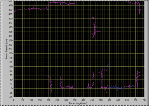
Figure 16. (a). Front panel view for 2D scanning and mapping; (b) Front panel view of the path traveled by robot
Computed servo motor and range finder information are used to find the 2D coordinates. Every point indicates the edge of the obstacle. The image processing can merge every edge of the obstacle, which is useful to identify the exact shape of the entire room or environment [2]. The number of obstacles at the robot path or indoor, which makes the success of the accurate mapping, can be slightly decreased [22]. Figure 16(a) and 16(b) show the graphical representation of the indoor mapping and robot path, respectively. This is one robot data that can extend into multiple robots simultaneously doing mapping with different locations data. All robot data are incorporated with the global position in the master computer [23]. This approach is one of the advanced technologies for localization and mapping which is used for automated guided vehicle development applications [2, 11].
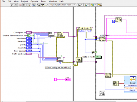
A network can be formed easily by an access point. In this case, a computer equipped with a wireless communication adapter is used. A software algorithm is developed to receive incoming data from the robot controller and perform the 2D simulation mapping [24]. Graphical representation of the software program is shown in Figure 17.
Figure 17. Graphical program for acquiring data from the mobile robot
(a)
Figure 18. (a) Single robot can perform mapping of the entire building; b). Multiple robots can simultaneously perform mapping at every room
Every robot has a separate address that it uses for localization identification and updating the 2D mapping of unknown area. Figure 18(a) shows the entire building mapping via a single robot. More robots can be used to survey the whole building with localization data. Figure 18(b) shows multiple robots simultaneously mapping every room. It reduces the mapping time to a single shot. Each robot has individual localizing and all data can be merged at the remote location for mapping the entire indoor environment. Figure 18(b) shows the front panel view of the experimental setup mapping data.
The efficient odometry method for the autonomous path planning stated in this research allows global optimal path planning, mapping, and localization in the presence of static obstacles of any shape. Local reconstruction of the robot’s position and orientation is made possible with an accurate calibration starting from the low-cost equipment. These improvements can easily be integrated into the global coordinate of a mobile robot using information from 2D and 3D mapping landmarks. It provides a consistent global map that can be used in the autonomous navigation of mobile robots. This research work used hardware implementation and odometry algorithm development. The experiments conducted showed good results, which suggests it an efficient odometry algorithm for increasing computing speed and position accuracy.
[1] Giovannangeli, C., Gaussier, P. (2010). Interactive teaching for vision-based mobile robots: A sensory-motor approach. IEEE Transactions on Systems, Man, and Cybernetics - Part A: Systems and Humans, 40(1): 13-28. https://doi.org/10.1109/TSMCA.2009.2033029
[2] Toda, Y., Kubota, N. (2013). Self-localization based on multiresolution map for remote control of multiple mobile robots. IEEE Transactions on Industrial Informatics, 9(3): 1772-1781. https://doi.org/10.1109/TII.2013.2261306
[3] Suh, J., You, S., Choi, S., Oh, S. (2016). Vision-based coordinated localization for mobile sensor networks. IEEE Transactions on Automation Science and Engineering, 13(2): 611-620. https://doi.org/10.1109/TASE.2014.2362933
[4] Censi, A., Franchi, F., Marchionni, L., Oriolo, G. (2013). Simultaneous calibration of odometry and sensor parameters for mobile robots. IEEE Transactions on Robotics, 29(2): 475-492. https://doi.org/10.1109/TRO.2012.2226380
[5] Lv, W., Kang, Y., Qin, J. (2019). Indoor localization for skid-steering mobile robot by fusing encoder, gyroscope, and magnetometer. IEEE Transactions on Systems, Man, and Cybernetics: Systems, 49(6): 1241-1253. https://doi.org/10.1109/TSMC.2017.2701353
[6] Martinez-Melchor, J.A., Jimenez-Fernandez, V.M., Vazquez-Leal, H., Filobello-Nino, U.A. (2018). Optimization of collision-free paths in a differential-drive robot by a smoothing piecewise-linear approach. Comp. Appl. Math., 37: 4944-4965. https://doi.org/10.1007/s40314-018-0602-x
[7] Antonelli, G., Chiaverini, S. (2007) Linear estimation of the physical odometric parameters for differential-drive mobile robots. Auton Robot, 23: 59-68. https://doi.org/10.1007/s10514-007-9030-2
[8] Barfoot, T.D., Clark, C.M. (2003). Motion planning for formations of mobile robots. Robotics and Autonomous Systems, 46(2): 65-78. https://doi.org/10.1016/j.robot.2003.11.004
[9] Choi, H., Yang, K.W., Kim, E. (2014). Simultaneous global localization and mapping. In IEEE/ASME Transactions on Mechatronics, 19(4): 1160-1170.
[10] Han, S., Kim, J., Myung, H. (2013). Landmark-based particle localization algorithm for mobile robots with a fish-eye vision system. IEEE/ASME Transactions on Mechatronics, 18(6): 1745-1756. https://doi.org/10.1109/TMECH.2012.2213263
[11] Son, J., Ahn, H. (2015). Formation coordination for the propagation of a group of mobile agents via self-mobile localization. IEEE Systems Journal, 9(4): 1285-1298. https://doi.org/10.1109/JSYST.2014.2326795
[12] Kim, J., Chung, W. (2016). Localization of a mobile robot using a laser range finder in a glass-walled environment. IEEE Transactions on Industrial Electronics, 63(6): 3616-3627. https://doi.org/10.1109/TIE.2016.2523460
[13] Barfoot, T.D., Clark, C.M., Rocks, S.M., D Eleuterio, G.M.T. (2002). Kinematic path-planning for formations of mobile robots with a nonholonomic constraint. Proceedings of the 2002 IEEE/RSJ International conference on Intelligent Robots and Systems, 3: 2819-2824. https://doi.org/10.1109/IRDS.2002.1041697
[14] Park, S., Roh, K.S. (2016). Coarse-to-fine localization for a mobile robot based on place learning with a 2-D range scan. IEEE Transactions on Robotics, 32(3):528-544. https://doi.org/10.1109/TRO.2016.2544301
[15] Meng, Q.H., Bischoff, R. (2004). Odometry based pose determination and errors measurement for a mobile robot with two steerable drive wheels. Journal of Intelligent and Robotic Systems, 41: 263-282. https://doi.org/10.1007/s10846-005-3506-0
[16] Choi, B.S., Lee, J.W., Lee, J.J., Park, K.T. (2011). A hierarchical algorithm for indoor mobile robot localization using RFID sensor fusion. IEEE Transactions on Industrial Electronics, 58(6): 2226-2235. https://doi.org/10.1109/TIE.2011.2109330
[17] Miah, M.S., Knoll, J., Hevrdejs, K. (2018). Intelligent range-only mapping and navigation for mobile robots. IEEE Transactions on Industrial Informatics, 14(3): 1164-1174. https://doi.org/10.1109/TII.2017.2780247
[18] Eberst, C., Andersson, M., Christensen, H.I. (2000). Vision- based door-traversal for autonomous mobile robots. Proceeding of the 2000 IEEE/RSJ International Conferences on Intelligent Robots and Systems, pp. 620-625. https://doi.org/10.1109/IROS.2000.894673
[19] Blanco, J.L., Fernández-Madrigal, J.A., Gonzalez, J.. (2008). A novel measure of uncertainty for mobile robot SLAM with Rao–Blackwellized particle filters. The International Journal of Robotics Research, 27(1): 73-89. https://doi.org/10.1177/0278364907082610
[20] Liu, M. (2016). Robotic online path planning on point cloud. IEEE Transactions on Cybernetics, 46(5): 1217-1228. https://doi.org/10.1109/TCYB.2015.2430526
[21] Chwa, D. (2016). Robust distance-based tracking control of wheeled mobile robots using vision sensors in the presence of kinematic disturbances. IEEE Transactions on Industrial Electronics, 63(10): 6172-6183. https://doi.org/10.1109/TIE.2016.2590378
[22] Cheon, H., Kim, B.K. (2019). Online bidirectional trajectory planning for mobile robots in state-time space. IEEE Transactions on Industrial Electronics, 66(6): 4555-4565. https://doi.org/10.1109/TIE.2018.2866039 https://doi.org/10.1109/TMECH.2013.2274822
[23] Lee, G., Chong, N.Y., Christensen, H. (2010). Tracking multiple moving targets with swarms of mobile robots. Intel Serv Robotics 3: 61-72. https://doi.org/10.1007/s11370-010-0059-2
[24] Chen, H., Sun, D., Yang, J., Chen, J. (2010). Localization for multirobot formations in indoor environment. IEEE/ASME Transactions on Mechatronics, 15(4): 561-574. https://doi.org/10.1109/TMECH.2009.2030584