Fares Bouriachi* | Hicham Zatla | Bilal Tolbi | Koceila Becha | Allaeddine Ghermoul
© 2021 IIETA. This article is published by IIETA and is licensed under the CC BY 4.0 license (http://creativecommons.org/licenses/by/4.0/).
OPEN ACCESS
Traffic jams and congestion in our cities are a major problem because of the huge increase in the number of cars on the road. To remedy this problem, several control methods are proposed to prevent or reduce traffic congestion based on traffic lights. There are few works using reinforcement learning technique for traffic light control and recent studies have shown promising results. However, existing works have not yet tested the methods on the real-world traffic data and they only focus on studying the rewards without interpreting the policies. In this paper, we proposed a reinforcement learning algorithm to address the traffic signal control problem in real multi-phases isolated intersection. A case study based on Algiers city is conducted the simulation results from the different scenarios show that our proposed scheme reduces the total travel time of the vehicles compared to those obtained with traffic-adaptive control.
traffic signal control, signalized intersection, adaptive systems, machine learning, SUMO simulation
In recent years, the city of Algiers has experienced a huge explosion in the national automobile park with one million three hundred thousand vehicles (1.3 million vehicles) and 1.4 daily trips per capita, and with the growth rapid transport demand with limited infrastructure capacity, urban congestion has become one of the major socio-economic problems in the life of road users in urban cities.
In Algeria, the urban roads of the main agglomerations have experienced, in recent years, significant and growing congestion due to strong growth in the national automobile fleet in 2018. According to the National Statistical Office (ONS), the automobile fleet in Algeria reached 6,418,212 vehicles in 2018, an increase of 4.15% compared to 2017, or the equivalent of 255,538 new vehicles. This explains the increase in demand for road traffic, around 85% of passenger movements are made by road and 90% of the volume of trade (internal transport of goods excluding transit) is carried out by road transport [1].
In this paper, recent advances in the field of artificial intelligence are used to research and develop a learning agent capable of controlling a traffic light system, with the aim of increasing the efficiency of road transport. The problem addressed in this thesis is defined as follows: given the state of a traffic light intersection, which phase of traffic lights should the officer choose in order to optimize traffic efficiency?
The remainder of the paper is organized as follows: section 2 we present a bereft stat of the art of work to control traffic problem. Section 3 presents the proposed agent design divided into state, action, reward, and learning mechanism. In section 4 we describe the agent training phase and the techniques used in this process, such as agent exploration strategy or traffic control algorithm. Section 5 is devoted to the performance evaluation of the proposed control strategy and that we will validate our results with an application by simulations on an intersection located in downtown Algiers in order to validate our results.
The Reinforcement learning have capability to provide a solution to Traffic signal control, this solution has recognized, displayed and validated by many authors and research studies the concept of reinforcement learning in traffic signal control are with deferent way: Harley et al. [2] proposed a conceptually simple and light weight framework for deep reinforcement learning that uses asynchronous gradient descent for optimization of deep neural network controllers, in [3] the describes using multi-agent reinforcement learning (RL) algorithms for learning traffic light controllers to minimize the overall waiting time of cars in a city, Wiering [4] made an introduction to Q-learning, a simple yet powerful reinforcement learning algorithm, and presented a case study involving application to traffic signal control. Reinforcement learning methods are applied for realistic and complex urban traffic network models [5]. Aslani et al. [6] use an organization called holonic multi-agent system (HMAS) to model a large traffic network.
The evolution in machine learning have produced a deep reinforcement learning techniques [7, 8] which have been applied for traffic signal control in many works [9, 10]. Authors [11-13] used the extensive reinforcement learning for traffic signal control provides a numerous possible state representations as: vehicle density, flow, queue, location, speed along with the current traffic phase, cycle length and red time.
In this section, we aim to improve the flow of traffic passing through an intersection controlled by traffic lights will be studied using learning techniques. The analysis will be carried out with a simulation where an agent manages the choice of the phase of activation of traffic lights with the objective of optimizing traffic efficiency. In order to choose the best light phase in each situation, a certain learning mechanism is required by the agent. The learning techniques used in this paper relate to reinforcement and deep learning. The whole system which includes the agent. The learning techniques used in this paper relate to reinforcement and deep learning. The whole system which includes the agent, its elements.
3.1 Problem definition
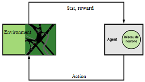
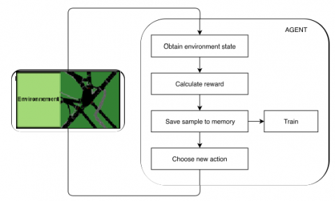
In this work, the environment is represented by a 4-lane intersection. A set of traffic lights (TL) manages the flow of traffic entering the intersection. Traffic signal control system (TSCS) is made up of a single agent that interacts with the environment using a state (s), an action (a) and a reward (r). A deep Q-Learning neural network is the learning mechanism of the agent. Figure 1 shows a summary of the TSCS.
Figure 1. TSCS work process
During the simulation, the agent takes samples from the environment and receives a state St and a reward r, where t is the current time step. According to the state and the prior knowledge, the agent chooses the next action which has the same time, the agent learns the consequences of the action taken in state using the reward and the state of arrival. The knowledge will be used to train the agent (i.e., neural network) to gain significant awareness of the consequences of future actions in similar states.
The problem is defined as follows: given the state of the intersection s, which is the phase a of the traffic lights that the agent must choose, chosen from a fixed set of predefined actions a, in order to maximize the reward r and optimize the efficiency of traffic at the intersection.
It should be noted that in this work, the possibility of a real application of the TSCS will be taken into consideration when designing the elements of the agent, in order not to use elements that might be difficult to implement with the technology currently available.
3.2 The simulation environment
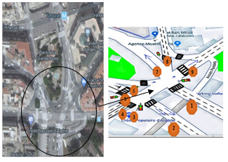
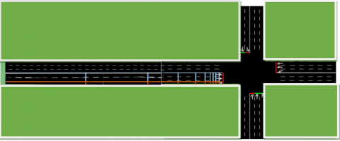
The simulated environment for this project is the intersection shown in Figures 2 and 3 It is a four-lane intersection. Each section of the junction is: [Colonel Amirouche Street 325 meters - Mohamed Khmisti Street 191 meters - AsselahHocine Street 462 meters - Sofia Parking Street 134 meters] long from the vehicle of origin to the stop line of the intersection.
On each section, the four lanes used to enter the intersection indicate the possible directions a car may take. When a vehicle approaches the intersection, it selects the desired lane depending on its destination:
Figure 2. Intersection geometry
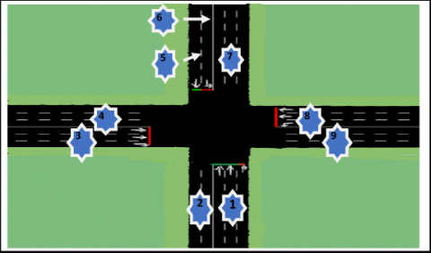
To facilitate work on this intersection, the spaces have been removed, in order to obtain normalized intersection, see Figure 3.
Figure 3. Intersection simplifies
3.3 The traffic light system
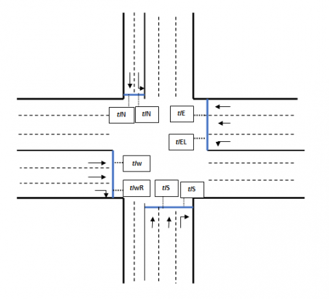
In the environment there are eight different traffic lights, each of them regulating one or more adjacent lanes. They are represented in Eq. (1).
$TL=\{t{{L}_{N}};t{{L}_{NG}};t{{L}_{W}};t{{L}_{WD}};t{{L}_{S}};t{{L}_{SD}};t{{L}_{E}};t{{L}_{EG}}\}$ (1)
where, the index indicates the position of each traffic light. For example, tLN is the traffic light that regulates all traffic from the north that wants to go straight. Alternatively, tLNG the regulates traffic coming from the north but only for vehicles that want to turn left. The same rule applies to each traffic light defined in set (1). A representation of each traffic and their position in the environment is shown in Figure 4.
Figure 4. Position of each traffic light in the environment
As with traditional traffic lights, a simulation tL traffic light has 3 possible states as described in set (2):
{Green, Red, Yellow} (2)
Each traffic light in the environment operates according to the following rules:
3.4 State representation
The state of the agent describes a representation of the situation of the environment in a given time step t and it is designated by st. To enable the officer to effectively learn how to optimize traffic, the State should provide sufficient information on the distribution of cars on each road.
The objective of this representation is to inform the agent of the position of the vehicles in the environment at the time step t. In particular, the design of this state includes only spatial information about the vehicles hosted in the environment, and the cells used to discretize the continuous environment are not regular.
In this project, we will examine the chances of achieving good results with a simple and easy to apply state representation. In each section of the intersection, the entry lanes are discretized into cells that can identify the presence or absence of a vehicle within. Figure 5 shows the state representation for the western section of the intersection.
Figure 5. Representation of the state in the west arm of the intersection
3.4.1 The discrete representation of the intersection
Formally, an IDR vector is defined as a discrete representation of the intersection (Intersection Discretized Representation) as the mathematical representation of the state space, where each element of IDRk is calculated according to Eq. (3).
$I D R_{k}=c_{k}$ (3)
where, ck is the k-nth cell. This means that each cell c is mapped to a position of the IDR vector. The IDR vector is updated according to rule (3).
IDRk = 1 if there is more than one vehicle inside ck=0 otherwise.
3.5 Set of action
The set of actions identifies the possible actions that the agent can take. The agent is the traffic light system, so taking an action result in turning the traffic lights green for a set of lanes and keeping it green for a fixed amount of time. The agent's task is to launch a green phase by choosing among those which are predefined. The action space is defined in the set (4).
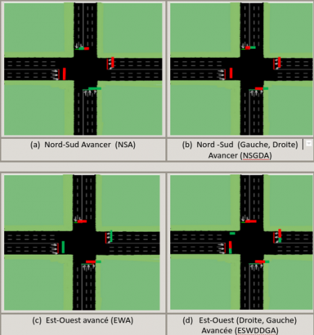
A = {NSA, NSGDA, EOA, ESODGA} (4)
The set represents all the possible actions that the agent can take. Each action has from the set (5) is described below.
Figure 6 below shows a visual representation of the 4 possible actions.
Figure 6. The four possible actions
3.6 The reward function
In reinforcement learning, the reward represents feedback from the environment after the agent chooses an action. The agent uses the reward to understand the outcome of the action taken and improve the pattern for the future of action choices. Therefore, reward is a crucial aspect of the learning process.
In this work the goal is to maximize the flow of traffic at the intersection over time. In order to achieve this goal, the reward must be calculated from a performance measure of traffic efficiency, so that the agent is able to understand whether the action taken will reduce or increase the efficiency of traffic. Intersections.
In traffic analysis, several measures are used, such as throughput, average delay and travel time. In traffic lights, several actions taken by the candidate to generate the reward were as follows.
Among the measures proposed, the measure chosen is total waiting time. Formally, the total waiting time is defined in Eq. (5).
$t w t_{t}=\sum_{v e h=1}^{n} w t_{(v e h, t)}$ (5)
where, tѡt_t is the total waiting time at step t and ѡt (veh, t) is the amount of time in seconds a vehicle has a speed less than 0.1 m / s at time step t. n represents the total number of vehicles present in the environment per time step t. The most efficient intersection is the one that prevents cars from waiting for the green phase. Therefore, the concept of wait time is crucial in choosing the reward metric. Total wait time is the most accurate measurement among those offered.
In the previous sections, the agent specification has been described, such as the state, possible actions and reward. Figure 7 shows how all these components work together to establish the agent's workflow during a single time step t.
Figure 7. The agent's workflow in a time step
After a fixed number of simulation steps, the agent's time step t begins. First, the agent recovers the state of the environment and the delay times. Then, using the delay times of time step t and the last time step t-1, it calculates the reward associated with the action taken at t-1. Then, the agent gathers the collected information and saves it in a memory which is used for training purposes. Finally, the agent chooses and fixes the new action to the environment and a new sequence of the simulation step begins. In this job, the agent is trained using micro-traffic simulator. The agent will be trained by submitting several episodes which consist of traffic scenarios, from which he will learn lessons. An episode consists of 5,400 steps, which corresponds to 1 hour and 30 minutes of the traffic simulation.
4.1 Experience replays
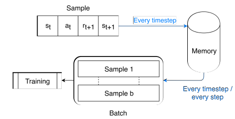
Experience replay is a technique adopted during the training phase in order to improve the performance of the agent and the learning efficiency. It consists of submitting to the agent the information needed for learning in the form of a randomized group of samples called batch, instead of immediately submitting the information that the agent gathers during the simulation (commonly called Online Learning).
Figure 8. The memory handling before training
The experience replay technique needs a memory, which is characterized by a memory size and a batch size see Figure 8. The memory size represents how many samples the memory can store and is set at 50000 samples. The batch size is defined as the number of samples that are retrieved from the memory in one training instance.
4.2 The training processes
This process is executed every time a training instance of the agent is initiated.
The training phase of the agent consists of finding the most valuable actions given a state of the environment. With that said, in the early stages of the training the agent does not know which actions are the most valuable ones. In order to overcome this problem, at the beginning of the training the agent should discover the consequences of the actions and do not worry about the performance. Once the agent has a solid knowledge about the action’s outcomes in a significant variety of states, it should increase the frequency of exploitative actions in order to find the most valuable ones and consequently increase the performance achieved in the task.
In our case study will reproduce 3 scenarios in order to better put the performance of the command into perspective, so we will use the following 3 cases:
In order to evaluate the performance of our agent, a set of fixed experiments was carried out on each trained agent. For each of the 3 scenarios randomly generated 1000 vehicles per episode with random directions. Then the agent is rated for each episode. Regarding the method used for the generated vehicles, we use Weibull's law in order to have a distribution with a car spike at a time t.
The evaluation is based on the following performance indicators:
$nr{{w}_{avg}}=av{{g}_{ep}}(\sum\limits_{t=0}^{nt}{nr{{w}_{t,ep}})}$ (6)
The sum of every negative reward nrw received at every timestep t in an episode ep, averaged among the 5 episodes.
$Twt=av{{g}_{ep}}(\sum\limits_{t=0}^{{}}{w{{t}_{veh,ep}})}$ (7)
The sum of the waiting times wt for every vehicle veh in an episode ep, averaged among the 5 episodes. Measured in seconds.
$Awt/v=media{{n}_{ep}}(\frac{\sum\limits_{wveh}{w{{t}_{veh,ep}}}}{\left| wveh \right|})$ (8)
The average wait time wt of those vehicles that have waited wveh, gathered from the episode with the median value of negative reward. Measured in seconds.
In this part, the experiments are carried out with fixed hyper parameters. These are described in Table 1. The main agent models tested are presented below. They are called Low Gamma Agent (LG), High Gamma Agent (HG).
Table 1. Fixed parameters
|
|
Low Gamma |
High Gamma |
|
NN structure |
5 Couches with 400 neurons |
5 Couches with 400 neurons |
|
Number of episodes |
100 |
100 |
|
Gamma |
0.1 |
0.8 |
The same neural structure was used for all the agents for the sake of training time, so we got suitable results with a 5/400 structure, however a deeper configuration could not be tested for the sake of training power. material used, so a 9-layer neuron network with 1000 neurons takes +800 seconds of training per episode, which is quite important considering that at least 100 episodes are required.
The choice of the neural structure used depends on two constraints: the desired performance and the total training time, which itself depends on the capacities of the machine used. Thus, for all the tests and simulations we will use the machine with the following characteristics:
The calculated training times are described in Table 2.
Table 2. Estimating the time required to train RNN
|
Training time |
RN simple 3 couches 200N |
RN simple 5 couches 400N |
RN simple 9 couches 1000N |
|
100 episodes |
7h |
10h |
28h |
|
1500 episodes |
90h |
112h |
18days |
For the simple neural network, the performance obtained is unusable and the training time is almost equal to the 5c / 400n neural network, and this is due to the fact that the small network cannot correctly map the acquired data. Regarding in-depth neural networks, the training time is much too long to be able to use it, solutions are offered in Cloud-Training, in particular with Google's CoLlab, but the latter is limited to 8 hours of training per project. And so, we will use the 5 hidden layers configuration with 400 neurons for each layer. Low and High agents use the literature reward function and an intense sampling strategy, but experiments show that this configuration is not beneficial for the agent with low gamma values.
5.1 Low Gamma
First, we used the model of an agent with a fairly low Gamma value (Low-Gama) that we trained with the hyper parameters represented in Table 2.
The size of the neural network is set to a starting value: variations in depth and width will be discussed later in this section.
The gamma is set to a low value: this means that the agent's anticipation is short and he will be more likely to prefer good immediate rewards, rather than waiting for a positive reward which could be acquired after more consequent actions. This agent behavior can be considered greedy.
After training, the result of negative rewards is shown in Figure 9. The latter represents the cumulative negative rewards.
Figure 9. Accumulate negative rewards
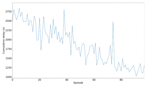
Figure 10. Cumulative waiting time
We notice that through the episodes, the accumulation of negative rewards does not converge towards a fixed value in a direct way. Sometimes the agent obtains an accumulation which is quite far from the neighboring values, especially during episode 37 and 70 with values -145000 and 178000 respectively, and this because the Gamma being low, he pushes the agent to seek a reward on the field which generally leads to poor traffic management, hence the points of divergence that can be seen in the graph in Figure 10.
Overall, however, we have fairly good performance on certain points, as can be seen from the previous graph. Thus, the cumulative waiting time per episode is improved compared to 50% of the initial departure time.
In summary, the agent with a Low Gamma performs well, except for the "High-traffic" scenario being the only one that is not very efficient, it will be a recurring event in each model of the agent tested.
This scenario causes long queues more than 200 cars on each lane because the number of cars generated is greater than the capacity of the junction. This explains the poor performance of the agent. When the agent sets a green phase where there is a long queue, starting the cars activates a wave of movement along the queue. This means that every waiting time for every car in the queue resets itself, but they don't happen instantly. For very long queues, the agent receives the reward for the last cars in the queue very late for the time when the transfer phase is activated.
After training the data see Table 3. There is a constant improvement in traffic management for the Low-Traffic scenario, with around 39% improvement in total waiting time and 69% in average time per vehicle during one episode compared to traffic light straigie system [14-16], in another. On the other hand, we have the opposite with a deterioration in performance for the High-Traffic scenario. This confirms our statements previously.
Table 3. Results after training with a Low-Gamma
|
|
Low traffic |
Improvement over STL |
High traffic |
Improvement over STL |
|
Total waiting time |
12102.2 |
+39.1% |
422377.2 |
-11% |
|
1500 episodes |
12.2 |
+69.2% |
121 |
-9.6% |
5.2 High Gamma
This time the gamma value is set to a high value, while the other parameters are still fixed. High gamma means that the agent aims to maximize the expected cumulative reward of multiple consecutive actions.
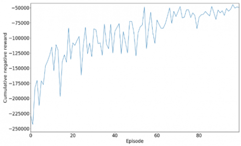
Figure 11. Evolution of cumulative negative rewards through episodes
This agent is best suited for road networks with a complex traffic influence, i.e. it can explore all the possibilities available to it in order to extract the best performance. Figure 11 represents the cumulative negative rewards obtained during training with low traffic.
We notice a clear improvement in the negative rewards in the queues of episodes, with a reduction from the latter to 75%. However, we also notice that towards the end of the training the agent tends to make less random decisions. In order to better understand the preceding graph, we must remember that during the training of the agent, the latter follows an epsilon exploration function. The more training progresses, the more the agent tends not to choose an exploration decision.
Therefore, it is normal that towards the start of the training, the agent performs poorly as he or she is more oriented towards exploratory actions. We notice that from episode 60 the cumulative negative rewards decrease with a decrease in the difference between the local max and the local minimum of the peaks of the graph, which means that the agent has learned a good decision-making policy in the first scenarios. An indicator of good training is stability towards the end of the graph.
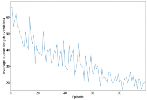
Figure 12. Cumulative waiting time
One of the performance criteria can be seen in Figure 12, we notice a clear decrease in the number of waiting cars, it goes from 65 cars on average to 20 cars which demonstrates the efficiency of the agent during his training in very beginning of the episodes. The different results are shown in Table 5.
Overall, there is an improvement of more than 50% in the total and average waiting time of each car compared to the STLS. As hoped, High-Gamma performs better compared to Low-Gamma and manages to reduce the waiting time to an average of 9 seconds. What is more interesting is to see an improvement in performance on the High-traffic side, however in order not to draw active conclusions it will be preferable to increase the number of episodes up to 1500 in order to see the real performance. of the agent in the face of high-traffic, because the observed improvement has not been robust enough (Table 4).
Table 4. Results after training with a High-Gamma
|
|
Low traffic |
Improvement over STL |
High traffic |
Improvement over STL |
|
N rewards |
-49824 |
- |
-220398 |
- |
|
Total waiting time |
8707.1 |
+56.2% |
365299 |
+4% |
|
Average waiting time |
8.9 |
+77.4% |
105 |
+3.9% |
Table 5. Numerical comparison between proposed control strategy and STLS
|
Objective function |
PCS |
STLS |
Improvement % |
|
Waiting time (s) |
38 |
71 |
46,6% |
|
Time lost(s) |
51.6 |
110 |
53.1% |
|
Co2(mg/s) |
83703.15 |
7032 |
47.3% |
|
Co (mg/s) |
76.10 |
127 |
40.1% |
|
Nox (mg/s) |
1.51 |
2.95 |
48.8% |
|
Bruit (Db) |
63.08 |
67.7 |
6.8% |
In the end, we better understand the impact of Gamma in the learning process, so for a better forecasting of future actions, an average Gamma is more suitable for urban traffic management, however the results obtained are the result of sufficient training. short of the agent, so that the latter can better learn the dynamics and stochasticity of the system, the latter must be trained over a longer period of time.
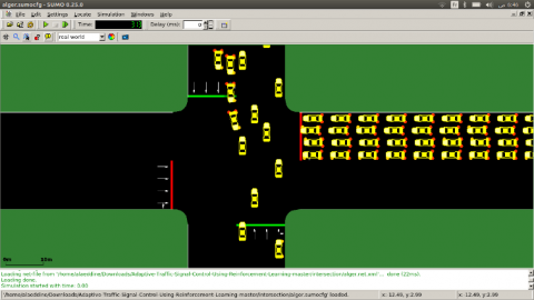
Figure 13. Simulation test under SUMO
The same problem has been investigated in Ref. [16] for the past year, who used a Genetic Algorithm to improve the performance of traffic management in the Sofia intersection. The comparative study Between proposed control strategy (PCS) and STLS are shown in Table 5.
According to Table 5, the results obtained from the experimental groups demonstrate (see Figure 13) that the application of Q-learning agent implemented in the context of signal traffic control in order to investigate the efficiency improvement compared with conventional methods.
In summary, the application of reinforcement learning techniques in the field of traffic light control is a difficult task, but with a very high potential. Multiple versions of the agent should be tested in order to find the appropriate state representation, set of actions, reward function, and learning techniques that allow the agent to perform best in each. traffic scenario.
In our case, the elements of the agent are defined in such so that the design is compatible with a real-world implementation. As well as the experimental results obtained presented and discussed have shown that the solutions proposed in our work surpass the classical methods.
In order to validate our results, we evaluated our control algorithm in simulations with the SUMO software. Our results demonstrate a drastic improvement in the wait time due to Q values generated by the deep neural network, compared to a traffic adaptive signal control.
Future research could be applied to the reinforcement learning techniques in large traffic network.
|
TL |
Traffic lights |
|
TSCS |
Traffic signal control system |
|
IDR |
Intersection Discretized Representation |
|
PSC |
proposed control strategy |
|
STLS |
straigie traffic ligth system STLS |
[1] https://www.tsa-algerie.com/parc-national-automobile-pres-de-6-millions-de-vehicules/ (cit. on p. 10).
[2] Harley, T., Silver, D., Kavukcuoglu, K., et al. (2016). Asynchronous methods for deep reinforcement learning. Proceedings of the 33rd International Conference on Machine Learning, pp. 1928-1937 http://dx.doi.org/10.5555/3045390.3045594
[3] Wiering, M.A. (2000). Multi-agent reinforcement learning for traffic light control. In Machine Learning: Proceedings of the Seventeenth International Conference (ICML'2000), pp. 1151-1158. http://dx.doi.org/10.1109/ITSC.2014.6958095
[4] Abdulhai, B., Pringle, R., Karakoulas, G.J. (2003). Reinforcement learning for true adaptive traffic signal control. Journal of Transportation Engineering, 129(3): 278-285. https://dx.doi.org/10.1061/(asce)0733-947x(2003)129:3(278)
[5] Jin, J., Ma, X. (2017), A group-based traffic signal control with adaptive learning ability. Engineering Applications of Artificial Intelligence, 65: 282-293. https://dx.doi.org/10.1016/j.engappai.2017.07.022
[6] Aslani, M., Mesgari, M.S., Wiering, M. (2017). Adaptive traffic signal control with actor-critic methods in a real-world traffic network with different traffic disruption events. Transportation Research Part C: Emerging Technologies, 85: 732–752. https://dx.doi.org/10.1139/cjce-2017-0408
[7] Lillicrap, T.P., Hunt, J.J., Pritzel, A., Heess, N., Erez, T., Tassa, Y., Wierstra, D. (2015). Continuous control with deep reinforcement learning. arXiv preprint arXiv:1509.02971.
[8] Rijken, T. (2015). DeepLight: Deep reinforcement learning for signalised traffic control (Doctoral dissertation, Master’s thesis. University College London).
[9] Rasheed, F., Yau, K.L.A., Low, Y.C. (2020). Deep reinforcement learning for traffic signal control under disturbances: A case study on Sunway city, Malaysia. Future Generation Computer Systems, 109: 431-445. https://dx.doi.org/10.1016/j.future.2020.03.065
[10] Li, L., Lv, Y., Wang, F.Y. (2016). Traffic signal timing via deep reinforcement learning. IEEE/CAA Journal of Automatica Sinica, 3(3): 247-254. http://dx.doi.org/10.1109/JAS.2016.7508798
[11] Genders, W., Razavi, S. (2016). Using a deep reinforcement learning agent for traffic signal control. arXiv preprint arXiv:161101142.
[12] Casas, N. (2017). Deep deterministic policy gradient for urban traffic light control. arXiv preprint arXiv:1703.09035.
[13] El-Tantawy, S., Abdulhai, B., Abdelgawad, H. (2014). Design of reinforcement learning parameters for seamless application of adaptive traffic signal control. Journal of Intelligent Transportation Systems, 18(3): 227-245. http://dx.doi.org/10.1080/15472450.2013.810991
[14] Bouriachi, F., Kechida, S. (2016). Hybrid petri nets and hybrid automata for modeling and control of two adjacent oversaturated intersections. Journal of Control, Automation and Electrical Systems, 27(6): 646-657. http://dx.doi.org/10.1007/s40313-016-0275-x
[15] Bouriachi, F., Tolbi, B., Saidi, K., Kloucha, O.K. (2019). Efficient traffic signal control for multi-phase intersections. In Proceedings of the 2019 International Conference on Artificial Intelligence, Robotics and Control, pp. 75-79. http://dx.doi.org/10.1145/3388218.3388223
[16] Bouriachi, F., Kechida, S. (2018). Modelling and analysis of oversaturated intersections using jointly hybrid Petri net and hybrid automata. International Journal of Intelligent Transportation Systems Research, 16(2): 138-150. http://dx.doi.org/10.1007/s13177-017-0144-4