Mohan Mahanty* | Debnath Bhattacharyya | Divya Midhunchakkaravarthy
© 2021 IIETA. This article is published by IIETA and is licensed under the CC BY 4.0 license (http://creativecommons.org/licenses/by/4.0/).
OPEN ACCESS
Colon cancer is thought about as the third most regularly identified cancer after Brest and lung cancer. Most colon cancers are adenocarcinomas developing from adenomatous polyps, grow on the intima of the colon. The standard procedure for polyp detection is colonoscopy, where the success of the standard colonoscopy depends on the colonoscopist experience and other environmental factors. Nonetheless, throughout colonoscopy procedures, a considerable number (8-37%) of polyps are missed due to human mistakes, and these missed polyps are the prospective reason for colorectal cancer cells. In the last few years, many research groups developed deep learning-based computer-aided (CAD) systems that recommended many techniques for automated polyp detection, localization, and segmentation. Still, accurate polyp detection, segmentation is required to minimize polyp miss out rates. This paper suggested a Super-Resolution Generative Adversarial Network (SRGAN) assisted Encoder-Decoder network for fully automated colon polyp segmentation from colonoscopic images. The proposed deep learning model incorporates the SRGAN in the up-sampling process to achieve more accurate polyp segmentation. We examined our model on the publicly available benchmark datasets CVC-ColonDB and Warwick- QU. The model accomplished a dice score of 0.948 on the CVC-ColonDB dataset, surpassed the recently advanced state-of-the-art (SOTA) techniques. When it is evaluated on the Warwick-QU dataset, it attains a Dice Score of 0.936 on part A and 0.895 on Part B. Our model showed more accurate results for sessile and smaller-sized polyps.
colonoscopy, colorectal polyp segmentation, computer-aided diagnosis (CAD), deep convolutional neural network, SRGAN
Colorectal cancer is growing rapidly throughout the world. As per the recent survey, colon cancer is diagnosed in 1,931,590 individuals, which is 10% of the total cancer cases [1]. Adenocarcinomas cause approximately 96% of colorectal cancers, and intestinal stromal tumors (GISTs). A polyp is a tiny development of excess cells, typically expands in the rectum or colon. All of the polyps may not turn into cancer cells, but it might take several years for a polyp to become malignant. The polyps can be detected through the standard biomedical imagining procedures such as Virtual colonoscopy, colon capsule endoscopy (CCE), and optical colonoscopy (OC) [2]. However, the wide variety of sizes and shapes of polyps and the minimal vision of the colon make it challenging to the endoscopists to maintain continual and regular assessments on detection and diagnosis of the polyps. In addition, recent scientific research studies have revealed that (8-37%) of polyps are missed as a result of high background object resemblance.
Over decades, computer vision-based techniques have been proposed for the automatic identification of polyps. Some researchers suggested utilizing the shape features and texture attributes combined with common classifiers for polyp detection. However, these techniques still struggle with a high False-positive rate. Recently, Deep CNNs have shown stupendous success in clinical image analysis, which can aid the colonoscopist to lower their polyp miss-rates in a real-time clinical atmosphere. The deep learning-based Encoder-Decoder network is an inexpensive tool used to segment a colorectal polyp effectively from the ubiquitously available histological images. However, automatic Polyp segmentation is challenging because of high variations in polyp appearance (texture, color, high interclass variations in size and shape), the presence of other endoluminal scene structures (e.g., colon walls and air bubbles), and the small multiple adenomas. Hence, developing an automated polyp segmentation system is necessary to support the gastroenterologists to identify and resect the polyps. The result is GAN-assisted Encoder-Decoder architecture. The contributions of this work are as follows.
We propose a novel GAN-assisted encoder-decoder architecture that is effective than compared with SOTA approaches.
We present an intelligent decoder design to ensure explicit contour preservation through GAN-assisted up-sampling processes at each decoder stage.
Our experimental results demonstrate noticeably better performance compared to current SOTA methods.
The remainder of the paper will be organized as follows. Section 2 explains the relevant work and the gap identification. Section 3 discusses the overview of CNN architecture, Encoder-Decoder network, and GANs. Section 4 introduces the suggested model, and Section 5 discusses the experimental results and analysis with SOTA techniques. Finally, the last section concludes the study in section 6.
Colon or colorectal cancer cases are increasing rapidly in developing countries. It affects the man more than women by 30 to 40%. A major rise in the frequency of colorectal cancer (CRC) was increasing the fatality rate. It is extensively approved that early detection and resects of polyps can prevent CRC. The well-known traditional method is colonoscopy, which consumes a lot of time and highly depends upon the colonoscopist experience. Computer system-assisted medical diagnosis of polyps helps radiologists to analyze the polyps.
Akbari et al. [3] proposed the FCNN based Polyp Segmentation from Colonoscopy Images. In the training phase, they used the patch selection method for the effective segmentation of polyps. By evaluating their classifier on the CVC-ColonDB dataset, they attain a dice score of 0.810. In Ref. [4], Nguyen and Lee proposed a consecutive Deep encoder-decoder network for polyp segmentation in the CVC-ColonDB dataset and attained a dice score of 0.896. Zhang et al. [5] used the hand-crafted and machine-learned features for polyp segmentation. On CVC-ColonDB, attain a dice score of 0.70. In Ref. [6], a CVC-ColonDB is used by the researchers for the segmentation of polyps using ResUNet++. When they evaluated the CVC-ColonDB, it attains a Dice similarity coefficient of 0.848.
Nguyen et al. [7] proposed the Detailed up-sampling based Encoder-Decoder Networks for Polyp Segmentations. However, when they evaluated the CVC-ColonDB, they attained a Dice score of 0.908. In Ref. [8], along with the Deep Neural Network, a Combination of Color Spaces are used for colon Polyp Segmentations. They trained the model by 80 % of the images and tested using 20 % of the images CVC-ColonDB dataset images and attained a Dice of 0.820. Thanh and Long [9] proposed their Segmentation model using the Ensembles of U-Nets with EfficientNet, and when they evaluated their model over the CVC-ColonDB, 0.891 Dice score. Feng et al. [10] proposed a novel network for Polyps segmentation in CVC-ColonDB, claimed that their model attains high performance with respect to Dice score of 92.97.
Researchers proposed various deep learning architectures for accurate polyp segmentation. They used various augmentation methods, features, and network models for accurate segmentation of colorectal polyps and reduced the poly miss rate. But if the model misses a polyp, it must be identified by the endoscopists traditionally. This shows the improvement is needed concerning the polyp miss rate. To surpass the SOTA methods, we propose a new up-sampling method using GAN, can effectively segment the colorectal polyps from colonoscopy images.
CNN [11] is a conventional deep neural network, basically used for object classification problems. The name convolution came from the linear mathematical operations between two matrices. CNN is composed by number of convolutional, pooling, non-linearity layers and is finally attached with a fully connected (FC) layer. The convolutional (conv) and FC layers have learnable parameters, but non-linearity and pooling layers do not have any learnable parameters. Generally, CNN concentrates on image classification problems, where input is an image (matrix) as well as output is one labeled image.
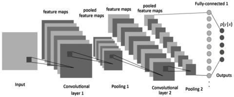
Figure 1. CNN architecture [12]
As depicted in Figure 1, in a CNN, a series of convolutional procedures are executed to generate the high-level feature maps from the given input image. Traditionally, the first Conv-Layer captures the Low-level features such as contours (edges), gradient orientation, color, etc. However, if the network is mode deeper, the additional Conv Layers adapt the high-level features as well, offering us the wholesome understanding of the processed images. After a series of Conv operations, pooling is performed, responsible for lowering the spatial size of the Convolved features.
In general, max-pooling is performed for image dimensionality reduction of the feature maps for suppressing the noise. For the given input feature map (Tensor), max-pooling gives the optimum value for the portion of the image overlapped by the kernel. After repeating the max pooling operations number of times, as shown in Figure 1, the design succeeds in recognizing the important features. After that, the final output is flattening as well as feed to an FCN for classification purposes. But in biomedical classification problems, along with the identification of disease is there or not, yet also to center the location of the abnormality. To accomplish this, there is a need for Encoder-Decoder based networks.
3.1 Encoder-decoder architecture
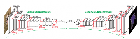
Figure 2. Encoder-Decoder Architecture [13]
Encoder-Decoder network evolved from the traditional convolutional neural network and can localize and identify contours of the objects by classifying each pixel in the image. As shown in Figure 2, in the architecture, the encoder (Left) part is also known as the contracting Path, which is comprised by the general convolutional procedure, and the Decoder (Right) part is also known as expansive Path, performs the Deconvolutions (Transposed convolutions), which seem to be the reverse of the encoder part.
3.2 Generative adversarial networks
Generative Adversarial Networks [14] (GAN) provide a path to innovative domain-specific data augmentation. Traditionally GAN [15] are a strategy to generative modeling making use of deep learning techniques. GANs use two neural networks Generator (G) and Discriminator (D). These two networks (G, D) play a min-max game where one attempts to outsmart the other network. The Generator is remained to be idle while the Discriminator is trained. In this phase, only forward propagation is done. The Discriminator is trained on original data for (n) number of epochs and sees if it can properly forecast them as original (real). Also, in this phase, the Discriminator is likewise trained on the phony (fake) generated data from the Generator (G) and saw if it can appropriately classify them as phony. The discriminator network (D) target is to determine which outputs it obtains have been artificially produced.
Figure 3. Basic Working model of GAN [16]
The goal of the generator network is to create synthesized data artificially and try to fool the Discriminator network. The Generator network is trained while the Discriminator remains idle. After the Discriminator network is trained by the phony data generated by the Generator, we can get its classification predictions and again use the outcomes to train the Generator network to improve from the previous state (more accurate fake data). The generated fake data is given to the discriminator network along with the original data. The Discriminator needs to classify the input images and returns a probability depend upon the loss function, between 0 and 1. This value represents the authenticity of each image. One (1) associate with original and zero (0) associates with phony images. If the loss is more, the output generated by the Discriminator (D) is again given back to the Generator (G) as input for fine-tuning. This process is repeated until the loss is minimized (The Discriminator fails to identify the fake data). Figure 3 represents the working functionality of a GAN.
The Generator G(z) attempts to reduce this loss function(min-max) value while the Discriminator tries to maximize it, which seems like a min-max game. Thus, Eq. (1) represents the min-max loss function, where Eq. (2) represents the loss at the Discriminator network D(x).
$ Min~\text{max}\left( D,G \right)$ (1)
${{E}_{x}}\left[ \log \left( D\left( x \right) \right) \right]+{{E}_{z}}\left[ \log \left( 1-D\left( G\left( z \right) \right) \right) \right]$ (2)
While the Discriminator classifies the original and phony images, if the loss is more with respect to the Generator, it needs to do back propagation in the Generator network. Both the networks are working adversarial to the other to generate the synthetic data, which can pass for original input data. Initially, GANs are used to generate fake images, which is similar to the original image. Researchers proposed that GANs can also be used mainly in the process of data augmentation. CycleGAN [17] is used to improve the generalizability in CT segmentation tasks. In Ref. [18], GANs are used for Semi-Supervised Semantic Segmentation, and SeGAN was proposed by Xue et al. [19] for Medical Image Segmentation.
In Ref. [20], SRGAN was used for image super-resolution, which surpassed the traditional up-sampling methods (nearest neighbor, bilinear interpolation, bicubic interpolation). Most of the GANs are used to generate the augmented image data used in the training phase of a CNN. To the best of our knowledge, this is the first study to use SRGAN [20] to substitute the traditional Up-sampling process at the decoder phase. The accuracy of the polyp segmentation depends upon the up-sampling process. Whereas the existing up-sampling methods have limitations in generating the accurate high-level segmented masks for the polyps. These drawbacks inspired us to develop an SRGAN assisted automatic Encoder-Decoder based model for accurate polyp detection and diminish the polyp miss rate from the colonoscopic images.
In a real-time environment, detection of the predecessor polyps is very difficult due to their shape (flat, sessile, sub-pedunculated, or pedunculated) and small size. Therefore, localization and identification of polyps play a crucial role in diagnosing colon cancer. Figure 4 depicts the proposed architecture consists of Encoder (Shrinking)- Decoder (extracting Path) for accurate polyp segmentation. The proposed encoder network comprises 11 convolutional layers, taken from the VGG16 network [21] and the corresponding Decoder network composed of the SRGAN.
4.1 Encoder
The proposed encoder network consists of 11 convolutional operations, organized into four levels. In the first level, two convolutional operations are performed by using the kernels (size 3 × 3, by stride 1) and generate the feature maps, which are then Group normalized [22] and element-wise Leaky ReLU [23] is applied. ReLU (Gives the value the results from max (0, x)) and zero for the negative values, yields to dead neuron problem. Leaky ReLU overcomes the dying ReLU Problem by additionally a small slope (small value say 0.001 (α)) for negative values instead of a flat slope. Eqns. (3) and (4) represents the functioning of Leaky ReLU.
$f\left( x \right)=\max \left( 0.001x,x \right)$ (3)
$f\left( x \right)=1(x<0)\left( \alpha x \right)+1(x>=0)$ (4)
At each level, after a set of convolutional operations, the generated feature maps [24] are transferred to the corresponding Discriminator (D) of the decoder network, used for the up-sampling process. Then they are sent into the max pooling [25] layer (2×2 size, stride 2) to diminish the input feature maps' size and generate the pooling indices, known as down-sampling. After down-sampling, the generated feature maps are given as input to the next-level convolutional layers for convolutional operations, but the numbers of kernels are doubled. The reduction of the spatial resolution of the feature maps reduced after every max-pooling operation can affect the segmentation process of the objects. To maintain the spatial information, need to transfer the obtained feature maps to the corresponding Decoder network.
Figure 4. Proposed architecture for polyp segmentation
4.2 Decoder
In Encoder decoder-based networks up-sampling process is performed repeatedly to enlarge the min-sized feature maps. All the existing networks use the transposed convolutions, Bilinear and Bicubic interpolations. However, when the GANs are used for the augmentation process, they generate far better results than the traditional interpolations [20]. Therefore, we utilized the SRGAN in the process of up-sampling.
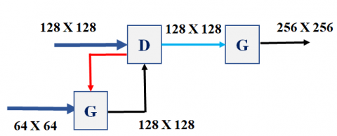
In the proposed model, the decoder network consists of 4 levels, and at each level, there is an SRGAN used for the up-sampling process. As shown in Figure 5, the feature maps (64X64) obtained from the encoder network (level 4) are given as input to the Generator (G) in the decoder network (Level-4), generates the more accurate feature maps (fake) of doubled size(128X128) and given as input to the Discriminator in the up-level (Level-3). The feature maps (128X128) of the level- 3 encoder block are given as input to the Discriminator. Now the generated output of the Discriminator network (Level-3) is given as input to the Generator network, which generates a double-sized fake image (256X256) and is given to the upper lever Discriminator network.
Figure 5. Up-sampling process at the decoder network
The new feature maps (Fake) generated by the Generator network and the feature maps from (Level -3) are given as input to the Discriminator, which needs to classify the fake and real feature maps. We considered the minimax GAN loss (Eq. (1)), where min is the generator (G) loss (Minimization), and max represents the discriminator (D) loss (maximization). As displayed in formula (5), always the Discriminator (D) wants to optimize the log probability of original (real) images and the log of inverted probabilities of phony images generated by the Generator.
$\text{maximize logD}\left( \text{x} \right)\text{+log}\left( \text{1-D}\left( \text{G}\left( \text{z} \right) \right) \right)$ (5)
As shown in Eq. (6), the Generator (G) wants to minimize the log of the inverse probability of fake images predicted by the Discriminator (D) (Eq. (6)). Thus, after fine-tuning, the Generator (G) can generate data with a very low probability of being fake.
$\text{minimize log}\left( \text{1-D}\left( \text{G}\left( \text{z} \right) \right) \right)$ (6)
If the Discriminator returns the value near 0, then the feature maps are needed to be fine-tuned by sending back to the Generator network. And this process is continued until the Discriminator gives the loss function value near to 1. To achieve this, we performed the fine-tuning operation (Epochs) 100 times at each level of the decoder network. Finally, the data generated at the level 1 discriminator (512X512) is given as input to a multi-class classifier layer (Softmax). The output generated from the soft-max classifier is a segmented mask of the colorectal polyp.
5.1 Dataset
We employ the two basic requirements when taking into consideration a dataset. First is the dataset must be publicly available and properly annotated. We used the publicly available colonoscopy CVC-ColonDB [26] dataset, which consists of a total of 380 colonoscopy frames of 574×500 pixel resolution has been generated extracted from 15 different colonoscopy videos. The sequences are from regular colonoscopies and were selected to represent as much variation in polyp appearance as possible. The CVC-ColonDB dataset is composed of frames from the 15 different video sequences containing at least one polyp. The whole dataset contains different shapes and sizes of polyps. In addition to each polyp image, the appropriate ground truth of the image is provided, which consists of a binary mask representing the area covered by the polyp in the image. We Also consider another benchmark dataset Warwick–QU [27, 28], to compare the efficiency with our previous work with the proposed model. The dataset primarily consists of 85 images in the training part and 80 images in the testing part.
5.2 Data augmentation
In real-time, due to the lack of medical image data, deep learning models face considerable difficulty in medical imagining compared to other object detection problems. Image Data augmentation plays a decisive role in enhancing the number of colon polyp images. This fixes the data deficiency problem, boosts the model's efficiency, and helps to diminish the under-fitting. The images are taken from the CVC-ColonDB dataset (380 images) are have a fixed size resolution of (574×500). After removing the canvas around each image, the complete dataset images are resized into (512 X 512). First, we applied the horizontal & vertical flip on the original dataset images to generate 760 augmented images. Then we applied various data augmentation techniques such as random contrast, random brightness, and random rotation (by 90°, 180°, 270°) to generate 6840 augmented images. To fit and evaluate the proposed deep learning model, the images are divided into training dataset consists of 5472 (80%) images and testing dataset consists of 1368 images (20%). There is no intersection of images between the train and the test dataset. And on the Warwick–QU dataset, the training dataset was only augmented.
5.3 Results and Discussion
There are some basic metrics to evaluate the performance of the proposed model’s implementation on the benchmark colorectal polyp datasets. We considered the essential statistical validation metric, the Dice similarity coefficient (DSC) to evaluate the segmentation accuracy of the model. These metric ranges between (0-1), where zero (0) indicates no overlap and one (1) indicates perfectly overlapping. Eq. (7) describes the dice coefficient at the pixel level. For segmentation tasks, we need to measure the dice index at the object level described in Eqns. (8) and (9).
$Dice\left( G,S \right)=2*\frac{\left| G\cap S \right|}{\left| G \right|+\left| S \right|}$ (7)
$\operatorname{Dice}_{o b j}(G, S)=\frac{1}{2} *\left[\begin{array}{l}n_{G} \gamma^{*} \operatorname{Dice}\left(G_{i}, S_{*}\left(G_{i}\right)\right) \\ \sum_{i=1}^{n}+\sum_{j=1}^{n_{S}} \sigma_{j} * \operatorname{Dice}\left(G_{*}\left(S_{j}\right), S_{j}\right)\end{array}\right]$ (8)
$\begin{align} & {{\gamma }_{i}}={}^{\left| {{G}_{i}} \right|}/{}_{\sum\nolimits_{p=1}^{{{n}_{G}}}{\left| {{G}_{p}} \right|}}, \\ & {{\sigma }_{j}}={}^{\left| {{S}_{j}} \right|}/{}_{\sum\nolimits_{q=1}^{{{n}_{S}}}{\left| {{S}_{q}} \right|}} \\ \end{align}$ (9)
After establishing the model, it is evaluated on the CVC-ColonDB and Warwick–QU benchmark datasets. Due to the existence of the GAN at each level of the decoder network, the proposed model requires high computational power and a huge amount of time for training the network. But it generates more accurate feature maps in the up-sampling process. Table 1 describes the performance evaluation of the various SOTA models with respect to the Dice score on CVC-ColonDB.
To review the performance of the suggested model on the benchmark Warwick–QU dataset, we considered the object-level Dice index (Dobj) for segmentation accuracy and the Hausdorff distance (Eq. (10)) to measure the shape similarity among the ground Truth (G) and segmented images(S). The smaller Hausdorff distance represents the maximal similarity among the borders of S and G.
Table 1. Comparison of SOTA models with the proposed model over CVC-ColonDB
|
Model |
Dice Score |
|
Akbari et al. [3] |
0.81 |
|
Nguyen and Lee [4] |
0.896 |
|
Zhang et al. [5] |
0.701 |
|
Jha et al. [6] |
0.848 |
|
Nguyen et al. [7] |
0.908 |
|
Bagheri et al. [8] |
0.82 |
|
Thanh and Long [9] |
0.891 |
|
Feng et al. [10] |
0.929 |
|
Proposed model |
0.948 |
$\text{H}\left( \text{G},\text{S} \right)=\max \left\{ \begin{align} & \underset{\text{x}\in \text{G}}{\mathop{\sup }}\,\underset{\text{y}\in \text{S}}{\mathop{\inf }}\,\text{d}\left( \text{x},\text{y} \right), \\ & \underset{\text{y}\in \text{s}}{\mathop{\sup }}\,\underset{\text{x}\in \text{G}}{\mathop{\inf }}\,\text{d}\left( \text{x},\text{y} \right) \\ \end{align} \right\}$ (10)
${{H}_{obj}}\left( G,S \right)=\frac{1}{2}*\left[ \begin{align} & \sum\nolimits_{i=1}^{{{n}_{G}}}{{{\gamma }_{i}}}*H\left( {{G}_{i}},{{S}_{*}}\left( {{G}_{i}} \right) \right)+ \\ & \sum\nolimits_{j=1}^{{{n}_{S}}}{{{\sigma }_{j}}}*H\left( {{G}_{*}}\left( {{S}_{j}} \right),{{S}_{j}} \right) \\\end{align} \right]$ (11)
Object wise Hausdorff distance (Hobj) is applied as shown in Eq (11) to find the object-wise contour-based shape similarity. The model achieved a dice score of 0.952 on Part A and 0.924 on Part B and Hobj of 76.142 (part A), 81.245(part B), which are more accurate than existing SOTA methods.
In this paper, we presented SRGAN-assisted Encoder-Decoder based deep convolutional model is discussed and evaluated for effective colorectal polyp semantic segmentation. The main motivation behind our proposed model was the need to design an efficient deep learning architecture for semantic segmentation of polyps from colonoscopy images. We analyzed the proposed model and compared with other bench mark model to reveal the practical trade-offs involved in designing architectures for semantic segmentation, particularly segmentation accuracy. Existed architectures uses the deconvoluted feature maps or max pooling indices or the encoder network feature maps in the decoder network, may consume less memory but the segmentation accuracy is less. The proposed model uses the Generative Adversarial Networks are used in up sampling process produces the dense feature maps, which increases the segmentation accuracy of the model. Our approach revealed good results in the segmentation of flat (sessile) and tiny polyps in a fully automatic manner from colonoscopic images, which are the significant factors for high polyp miss-rates. The model is well-acquainted with the benchmark colorectal datasets, consists of different dimensionalities of optical colonoscopy images. The implementation results of the suggested model are promising in terms of both illustrative contributions and experimental evaluations. The GANs in the model may consume huge time for training, but produce the most accurate results suggests that our method should be explored further for usage in medical image analysis.
[1] PRESS RELEASE N° 292. (2020). https://gco.iarc.fr/, accessed on Jun. 29, 2021.
[2] Misawa, M., Kudo, S.E., Mori, Y., Hotta, K., Ohtsuka, K., Matsuda, T., Mori, K. (2021). Development of a computer-aided detection system for colonoscopy and a publicly accessible large colonoscopy video database (with video). Gastrointestinal Endoscopy, 93(4): 960-967. http://dx.doi.org/10.1016/j.gie.2020.07.060
[3] Akbari, M., Mohrekesh, M., Nasr-Esfahani, E., Soroushmehr, S.R., Karimi, N., Samavi, S., Najarian, K. (2018). Polyp segmentation in colonoscopy images using fully convolutional network. In 2018 40th Annual International Conference of the IEEE Engineering in Medicine and Biology Society (EMBC), pp. 69-72. http://dx.doi.org/10.1109/EMBC.2018.8512197
[4] Nguyen, N.Q., Lee, S.W. (2019). Robust boundary segmentation in medical images using a consecutive deep encoder-decoder network. IEEE Access, 7: 33795-33808. http://dx.doi.org/10.1109/ACCESS.2019.2904094
[5] Zhang, L., Dolwani, S., Ye, X. (2017). Automated polyp segmentation in colonoscopy frames using fully convolutional neural network and textons. In Annual Conference on Medical Image Understanding and Analysis, pp. 707-717. http://dx.doi.org/10.1007/978-3-319-60964-5_62
[6] Jha, D., Smedsrud, P.H., Johansen, D., de Lange, T., Johansen, H.D., Halvorsen, P., Riegler, M.A. (2021). A comprehensive study on colorectal polyp segmentation with ResUNet++, conditional random field and test-time augmentation. IEEE Journal of Biomedical and Health Informatics, 25(6): 2029-2040. http://dx.doi.org/10.1109/JBHI.2021.3049304
[7] Nguyen, N.Q., Vo, D.M., Lee, S.W. (2020). Contour-aware polyp segmentation in colonoscopy images using detailed upsamling encoder-decoder networks. IEEE Access, 8: 99495-99508. http://dx.doi.org/10.1109/10.1109/ACCESS.2020.2995630
[8] Bagheri, M., Mohrekesh, M., Tehrani, M., Najarian, K., Karimi, N., Samavi, S., Soroushmehr, S.R. (2019). Deep neural network based polyp segmentation in colonoscopy images using a combination of color spaces. In 2019 41st Annual International Conference of the IEEE Engineering in Medicine and Biology Society (EMBC), pp. 6742-6745. http://dx.doi.org/10.1109/EMBC.2019.8856793
[9] Thanh, N.C., Long, T.Q. (2020). Polyp segmentation in colonoscopy images using ensembles of U-nets with efficientnet and asymmetric similarity loss function. In 2020 RIVF International Conference on Computing and Communication Technologies (RIVF), pp. 1-6. http://dx.doi.org/10.1109/RIVF48685.2020.9140793
[10] Feng, R., Lei, B., Wang, W., Chen, T., Chen, J., Chen, D. Z., Wu, J. (2020). SSN: A stair-shape network for real-time polyp segmentation in colonoscopy images. In 2020 IEEE 17th International Symposium on Biomedical Imaging (ISBI), pp. 225-229. http://dx.doi.org/10.1109/ISBI45749.2020.9098492
[11] Albawi, S., Mohammed, T.A., Al-Zawi, S. (2017). Understanding of a convolutional neural network. In 2017 International Conference on Engineering and Technology (ICET), pp. 1-6. http://dx.doi.org/10.1109/ICENGTECHNOL.2017.8308186
[12] Albelwi, S., Mahmood, A. (2017). A framework for designing the architectures of deep convolutional neural networks. Entropy, 19(6): 242. http://dx.doi.org/10.3390/E19060242
[13] Image segmentation with Deep learning - machine Intelligence. https://www.hackevolve.com/image-segmentation-using-deep-learning/, accessed on Jul. 18, 2021.
[14] Goodfellow, I., Pouget-Abadie, J., Mirza, M., Xu, B., Warde-Farley, D., Ozair, S., Bengio, Y. (2021). http://www.github.com/goodfeli/adversarial
[15] Goodfellow, I., Pouget-Abadie, J., Mirza, M., Xu, B., Warde-Farley, D., Ozair, S., Bengio, Y. (2014). Generative adversarial nets. Proceedings of the 27th International Conference on Neural Information Processing Systems, 4: 2672-2680.
[16] Gharakhanian, A. (2017). Generative adversarial networks-hot topic in machine learning. https://www.kdnuggets.com/2017/01/generative-adversarial-networks-hot-topic-machine-learning.html, accessed on Jul. 14, 2021.
[17] Sandfort, V., Yan, K., Pickhardt, P.J., Summers, R.M. (2019). Data augmentation using generative adversarial networks (CycleGAN) to improve generalizability in CT segmentation tasks. Scientific Reports, 9(1): 1-9. http://dx.doi.org/10.1038/s41598-019-52737-x
[18] Souly, N., Spampinato, C., Shah, M. (2017). Semi supervised semantic segmentation using generative adversarial network. In Proceedings of the IEEE International Conference on Computer Vision, pp. 5688-5696. http://dx.doi.org/10.1109/ICCV.2017.606
[19] Xue, Y., Xu, T., Zhang, H., Long, L.R., Huang, X. (2018). Segan: Adversarial network with multi-scale l 1 loss for medical image segmentation. Neuroinformatics, 16(3): 383-392. https://doi.org/10.1007/s12021-018-9377-x
[20] Ledig, C., Theis, L., Huszár, F., Caballero, J., Cunningham, A., Acosta, A., Shi, W. (2017). Photo-realistic single image super-resolution using a generative adversarial network. In Proceedings of the 30th IEEE Conference on Comput Vis Pattern Recognition, CVPR, pp. 105-114. http://dx.doi.org/10.1109/CVPR.2017.19
[21] Simonyan, K., Zisserman, A. (2014). Very deep convolutional networks for large-scale image recognition. arXiv preprint arXiv:1409.1556. http://www.robots.ox.ac.uk/.
[22] Wu, Y., He, K. (2002). Group normalization. International Journal of Computer Vision, 128(3): 742-755. https://doi.org/10.1007/978-3-030-01261-8_1
[23] Maas, A.L., Hannun, A.Y., Ng, A.Y. (2013). Rectifier nonlinearities improve neural network acoustic models. In Proc. ICML, 30(1): 3. https://doi.org/10.1.1.693.1422
[24] Ronneberger, O., Fischer, P., Brox, T. (2015). U-net: Convolutional networks for biomedical image segmentation. In International Conference on Medical Image Computing and Computer-Assisted Intervention, pp. 234-241. http://dx.doi.org/10.1007/978-3-319-24574-4_28
[25] Nagi, J., Ducatelle, F., Di Caro, G.A., Cireşan, D., Meier, U., Giusti, A., Gambardella, L.M. (2011). Max-pooling convolutional neural networks for vision-based hand gesture recognition. In 2011 IEEE International Conference on Signal and Image Processing Applications (ICSIPA), pp. 342-347. http://dx.doi.org/10.1109/ICSIPA.2011.6144164
[26] Bernal, J., Sánchez, J., Vilarino, F. (2012). Towards automatic polyp detection with a polyp appearance model. Pattern Recognition, 45(9): 3166-3182. http://dx.doi.org/10.1016/j.patcog.2012.03.002
[27] Sirinukunwattana, K., Pluim, J.P., Chen, H., Qi, X., Heng, P.A., Guo, Y.B., Rajpoot, N.M. (2017). Gland segmentation in colon histology images: The glas challenge contest. Medical Image Analysis, 35: 489-502. http://dx.doi.org/10.1016/j.media.2016.08.008
[28] Sirinukunwattana, K., Snead, D.R., Rajpoot, N.M. (2015). A stochastic polygons model for glandular structures in colon histology images. IEEE Transactions on Medical Imaging, 34(11): 2366-2378. http://dx.doi.org/10.1109/TMI.2015.2433900