Lince Rachel Varghese* | K. Vanitha
© 2021 IIETA. This article is published by IIETA and is licensed under the CC BY 4.0 license (http://creativecommons.org/licenses/by/4.0/).
OPEN ACCESS
This paper introduces the Q-learning-based deep reinforcement learning (Q-DRL) to the recurrent neural network (RNN) of the convolutional neural network-RNN (CNNRNN) model, aiming to improve the efficacy of rubber yield prediction based on optimum reward cycles under uncertainties, while interpreting ambiguous inputs accurately. The system builds a deep recurrent Q-network (DRQN) with the Q-DRL algorithm. The layers of CNNRNN were stacked in series, and then given the input variables. Based on these variables, the Q-learning network creates a rubber yield estimation model during training, by linearly mapping CNNRNN outputs to Q-factors. Then, the RL agent combines parametric attributes with a threshold to assist with rubber yield prediction. Further, the agent accepts an overall rate for the actions executed to minimize error and maximize forecast accuracy. If the time series is too long, however, the DRL-based RNN might suffer vanishing gradients. To solve the problem, probabilistic modeling schemes, such as data analytics, and probabilistic bias-difference decomposition, were introduced to the DRL to deal with the inherent ambiguity in geometric estimations. After that, the model predictive control (MPC) learns a probabilistic shift method utilizing Gaussian processes (GPs). Then, the MPC was applied to obtain a control series to minimize the predicted long-term cost. Because MPC enables the trained system to be restructured instantly, our method, denoted as CNNRNNPCDRL, became more robust to model inaccuracies.
convolutional neural network – recurrent neural network (CNNRNN) model, deep recurrent Q-network (DRQN), model predictive control (MPC), Gaussian processes (GPs), rubber yield forecast
Hevea brasiliensis (Pará rubber tree) is a significant industrial crop that occupies about 10 million hectares of the Earth's terrestrial surface [1], and generates over 11 million tons of natural rubber each year. For accurate forecast of rubber yield, the latex is often extracted repeatedly from the same rubber trees. If the interest lies in latex yield per harvest, it would be inevitable to collect data with the same measurement units from rubber trees across time. Considering the autocorrelation between rubber yields, mixed models must be adopted to process the sequentially correlated longitudinal data.
The rubber yield can be improved, if the weather is favorable, the vegetation is suitable, and the field conditions are close to the natural living environment. The ontology rubber model [2] offers a way to locate the suitable rubber cropland, in the light of every agro-climatic factor. With the aid of this model, it is possible to judge whether a field is suitable for rubber production, and predict rubber yield accurately, laying the foundation for sustained growth of rubber yield.
Deep neural networks (DNNs) help to predict and check yield, and identify the variation of rubber yield with genomes and weather conditions. As a kind of learning model, DNNs can automatically discover the underlying data representation, eliminating the need for manual feature input. A typical DNN consists of several nonlinear layers that convert the raw input into complex and sophisticated representations [3]. In this way, the system becomes deeper and more complex, and capable of obtaining precise results.
Khaki et al. [4] have hybridized convolutional neural network (CNN) with recurrent neural network (RNN) into CNNRNN model to predict crop yield based on environmental factors and management activities. The CNNRNN structure used to be introduced to derive rubber yield from three important influencing factors. The structure can capture the time dependency of environmental factors, shorten the computing time, and generalize the precise yield under uncertain conditions, without sacrificing the prediction accuracy.
In the CNNRNN model, the features are selected through error backpropagation, and the impact of each weather/soil condition is evaluated against yield. However, the RNN is prone to problems like vanishing or exploding gradients. During each iteration of training, the weight of each network node is updated according to the incomplete derivative of the error of the current weight. The gradient might be vanishingly small in some cases, making it impossible to modify the weight range. Exploding gradients are a problem that node weights are adjusted excessively during network training, due to the accumulation of a huge error gradient.
In this paper, the RNN in RNNCNN model is improved by recalling long-term inputs by long short-memory network (LSTM) cells, which are precisely constructed recurrent nodes that perform excellently in series modeling. In addition, a Q-learning-based deep reinforced learning (Q-DRL) system was employed in the RNN to realize efficient forecast of rubber yield with the best rewarding iterations. Then, a deep recurrent Q-network (DRQN) framework was built on Q-DRL for efficient crop prediction. Data parameters were fed into the sequentially stacked layers of CNNRNN. Based on the input variables, the Q-learning network generated a rubber yield forecast setting. Then, the CNNRNN results were mapped to Q-factors on a linear layer. After that, the rubber yield was estimated by including a mixture of parameterized attributes with a threshold into the reinforcement-learning agent. Eventually, the agent summarized the measures to eliminate errors, and evaluate forecast efficiency.
DRL-based RNN employs probabilistic analytical modelling schemes (e.g., data analytics and probabilistic bias-difference decomposition) to control the ambiguity in geometric estimations. In this paper, a model predictive control (MPC) was developed based on DRL probabilistic learning to integrate system ambiguity, fuse long-term forecasts, and reduce the effect of system error. After that, the MPC learns a probabilistic shift method utilizing Gaussian processes (GPs). Then, the MPC was applied to obtain a control series to minimize the predicted long-term cost, and realize real-time update of the learned model. In this way, our method, denoted as CNNRNNPCDRL, became more robust to model inaccuracies.
Haque et al. [5] proposed a DNN approach for crop yield forecast and checking, and yield dissimilarity identification based on genetics and weather information. Initially, the missing values in the environmental dataset were padded through median imputation. Next, two DNNs were trained to provide the gap between predicted and actual crop yields. The proposed DNN could understand the complex relationship between environmental conditions and crop genes, and estimate the yield for novel hybrid crops in unknown site according to climate conditions. However, the DNN is too complex for hypothesis test.
To predict crop yield accurately, Kalaiarasi and Anbarasi [6] designed a multi-parametric DNN (MDNN) to model the effects of climate change, weather condition, and soil parameters. Firstly, the growing degree day (GDD) was introduced to measure the overall effect of weather conditions on crop yield. The weather conditions were predicted by a neural network based on the collected dataset. After that, the predicted weather conditions, together with climate, and the impact of climate and soil parameters, were imported to a DNN. To improve the prediction effect, the leaky rectified linear unit (LeakyReLU) was implemented as the activation function of the MDNN. The problem with the MDNN lies in the difficulty of computation.
Anjula et al. [7] mined spatial data with the optimal neural network (ONN), and predicted crop yield in three steps: preprocessing, feature selection and prediction. The preprocessing generates a better model; the features were selected through multi-linear principal component analysis (MPCA); the crop yield was predicted with ONN classifiers. Nevertheless, they failed to evaluate the precision of the predicted results.
Using a hybrid adaptive neural genetic network, Qaddoum et al. [8] developed a framework for accurate crop yield prediction. Specifically, an intelligent computing technique was used as a learning system to forecast weekly tomato yield, with the environmental variables inside the greenhouse as the inputs. Following a modified optimizer approach, the connection weights of the neural network were adjusted through training. The convergence error of the network was examined in details. Nonetheless, the proposed framework has a low accuracy.
Bu and Wang [9] created a DRL model of four layers, namely, a farming information acquisition layer, an Internet of things (IoT) layer, an information dissemination layer, and a data storage layer, and combined the model with sophisticated technology to improve crop yield. The real-time agricultural demand of irrigation water was determined smartly, with the help of artificial intelligence (AI) and extensive training. But the training phase was sluggish in getting the exact results.
The remainder of this paper is organized as follows: materials and methods, results and discussion, and conclusions.
3.1 Data acquisition
This research aims to improve the prediction accuracy of rubber yield in Kerala, a southwestern coastal state of India. The potential factors affecting rubber yield, such as soil, rainfall, humidity, temperature, and average wind speed, were acquired from the India Metrological Department [10], and the data published by the Rubber Institute of India (RRII) [11], Kottayam. Multiple soil parameters were studied, including pH, organic carbon, phosphorus, potassium, calcium, iron, boron, etc.
To predict rubber yield, the data on the above factors from 2018 to 2021 were collected from different districts of Kerala, namely, Alappuzha, Ernakulam, Kannur, Idukki, Kasargode, Kollam, Kottayam, Kozhikode, Palakkad, Pathanamthitta, Thiruvananthapuram, Thrissur, and Wayanad.
3.2 Proposed CNNRNN Model
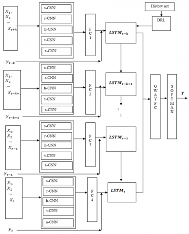
Figure 1. Structure of our CNNRNN model
The DRL has evolved over the time through data expansion and measurement improvement, as new ways emerge to determine, evaluate, and recognize the data process in rubber yield forecast frameworks. The prediction of rubber yield must fully consider the constantly changing factors. This paper initializes a CNN for the spatiotemporal changes of each feature: soil, rainfall, humidity, temperature, and average wind speed. These one-dimensional (1D) CNNs are abbreviated as s-CNN, r-CNN, h-CNN, t-CNN, and a-CNN, in turn. The high-level features extracted by the above CNNs were fused on a fully connected layer (FC) to reduce the dimensionality.
Based on the data on previous years (t-k, t-k+1, …, t-k, t), the RNN, which was augmented with CNN structure, was adopted to estimate the rubber yield of a certain state in year t. The mean yield data of all states in the same year, management data, and FC layer performance were imported to the cell, which derives the fundamental features processed by the said CNNs.
The DRL, Q-learning, and deep Q-network (DQN) frameworks for rubber yield forecast are detailed in this subsection. Figure 1 shows the structure of our CNNRNN model. The DRL is embedded in the structure to enhance the accuracy of yield prediction.
3.3 Reinforcement learning (RL)
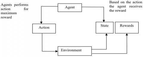
As an AI paradigm, RL builds and trains strategies with an incentive and penalty system through adaptive programming [12]. During the RL, the problem is usually solved by Markov selection. The agent-like RL algorithm learns through cooperation and interaction with the surroundings. The agent would be rewarded for correct actions, and penalized for incorrect actions. The learning requires no manual intervention, for the agent automatically pursues a higher reward and a lower penalty. In our model, an agent in state ‘s’ (rubber yield prediction) takes an action ‘a’ (soil, rainfall, humidity, temperature, and average wind speed). After the action is completed, the agent receives a reward R(s, a), and enters a new state ‘s’. The mapping criteria between states and actions are called rules. In each state, a rule $\pi$ is calculated to define the agent’s action. Here, there are three possible states: low, medium, and high. Once a parameter value changes, the rule under which the crop yield can be predicted with the minimum error is considered the best rule for that parameter. Throughout its lifespan, the agent aims to find the best rule $\pi *$ that maximizes the overall low-cost incentive.
The best rule can be depicted as:
$\pi *(s)=\underset{a \in A}{\operatorname{argmax}} \sum_{s^{\prime} \in S} P_{s a}\left(s^{\prime}, a\right) V^{*}\left(s^{\prime}, a\right)$ (1)
For each state-action combination, a value factor $V^{\pi}(s, a)$ [13] was introduced to represent the forecast of the predicted incentive following $\pi$. The best rule, which is determined by the maximum incentive gained by the agent in each state, yields the optimal value factor:
$V^{*}(s, a)=R(s, a)$$+\max _{a \in A} \gamma \sum_{s^{\prime} \in s} P_{s a}\left(s^{\prime}, a\right) V^{*}\left(s^{\prime}, a\right)$ (2)
In this way, each RL agent is trained through the interaction with the surroundings. Through dynamic programming, every RL agent optimizes his/her benefits to find the best rule and value factor. Figure 2 illustrates the RL process.
Figure 2. RL process
3.4 Q-learning
The QL, as a way to determine the actions of an agent depending on a value-action factor, computes the probability for an action to occur in a given state. One of the most substantive advances in RL is the introduction of a non-political method called temporal variance management. To identify the most valuable action for a target policy, Q-learning assesses the condition-action range factor. With the current state (s) and action (a) as inputs, the Q function predicts the incentive, and provides arbitrary fixed values in the first step of configuration assessment.
3.5 DQN
DQN is an extended RL agent with DNN. It is comparable to a Q-table in QL, which records the mapping relationship between states and actions. Typical examples of DNNs capable of directly learning abstract representations from raw data include CNN, RNN, and sparse autoencoders. There is virtually no difference between a DQN agent and a Q-learning agent in the communication with the environment via a series of observations, actions, and benefits. The two serve the same task, for many annotations, activities and incentives adopt the DQN structure. During the improvement of the DQN agent, an understanding is randomly selected from storage to continue the process, and RNN is taken as the DQN to estimate the factor with weight $\theta$. As a result, the Q-network can be established by reducing the mean squared error (MSE) in the Bellman equation by adjusting variable $\theta_{i}$ in the i-th iteration.
The loss, i.e., the squared variance between the desired Q and the estimated Q, can be defined as:
$Loss=\left(r+\gamma_{a^{\prime}}^{\max } Q\left(s^{\prime}, a^{\prime} ; \theta^{\prime}\right)-Q(s, a ; \theta)\right)^{2}$ (3)
Gradient descent for the real variables is adopted to mitigate this loss.
3.6 DRL for CNNRNN
The DRL-based crop yield monitoring can be understood with the input parameter that converts supervised learning into RL. The surroundings need to be determined through prediction games, each of which consists of the mixture of parameterized attributes and a threshold. The attributes contribute to crop production. At the beginning of the game, the agent performs tasks to get rewards on the value of crop yield. If the value falls in the desired range, the agent would receive a positive incentive; otherwise, it will receive a negative incentive.
Normal RL techniques like QL cannot easily discriminate and analyze yield predictions, owing to their limitations in state definition. By virtue of the strength of DQN in big data analysis, this paper employs a CNNRNN to estimate rubber yield based on various factor, such as soil, rainfall, humidity, temperature, and average wind speed. The CNNRNN is sophisticated enough to mine spatiotemporal and lexical features in forecast, language modeling, and voice recognition. As a variant of artificial network, the CNNRNN combines the input of the current state with the output of the previous state to determine the results. Briefly speaking, the network can recall earlier data, and use them in the calculation of the current state.
The DQN agent was created by stacking the CNNRNN layers sequentially, initializing the network parameters through pre-learning, and adding a linear layer that maps the RNN results to $\mathrm{Q}$ scores. Let $x^{t}$ be the input of the learning sample at time $\mathrm{t} ; \mathrm{H}^{\mathrm{t}}$ be the hidden layer state at time $\mathrm{t}$, which depends on the current input $x^{t}$ and the previous hidden layer state $H^{t-1} ; O^{t}$ be the result of the current layer at time t; $L$ be the error at time $\mathrm{t}$, which depends on the learning sample output $Y^{t}$ and the current layer output $O^{t} ; u, v$, and $w$ be the weights of the CNNRNN; $b_{1}$ and $b_{2}$ be the mutual RNN thresholds. Then, the range of hidden layer state at time $t$ can be calculated by:
$H^{t}=f\left(u \times x^{t}+w \times H^{t-1}+b 1\right)$ (4)
The expected output $0^{t}$ of the RNN at time $t$ can be calculated by:
$O^{t}=f\left(v \times H^{t}+b 2\right)$ (5)
The error L of the RNN can be calculated by:
$L=O^{t}-y^{t}$ (6)
The RNN can effectively compute crop yield, because the space variable and overfitting are restricted by two factors: the layered description of original features and the sparse constraint. Every learning instance is pre-learned before DRL. Then, the agent forecasts the yield to generate Q-range layer by layer.
DRL training involves so many states and actions that the correlations between data might be unstable. Therefore, two adjustments were made to the DQN training. The primary adjustment is understanding replay: the agent’s understanding is preserved in the replay storage (D) using the state, action, and reward of the current timestamp, as well as the state of the next timestamp. This adjustment saves the agent’s understandings. Individual understanding $e_{t}$ at $t$ are characterized as $e_{t}=\left(e_{t}, x_{t}, a_{t}, r_{t}, s_{t+1}\right)$, and the memories time at $t$ are denoted as $D_{t}=\left\{e_{1} \ldots . . e_{t}\right\}$. Experience replay is a useful technique for eliminating parameter divergence, allowing agents to distinguish their understanding through training. The next adjustment is to allow an autonomous system to generate the goals during QL upgrading. Through the adjustments, DRL training becomes much more stabler.
Note that most RL strategies employ a Bellman equation to iteratively update the action value factor. The updating process is rather time consuming. To solve the problem, this paper predicts this factor by the weighted RNN predictor with weight $\theta$. Hence, the Q-network can be produced by decreasing the MSE in the Bellman equation by revising parameter $\theta_{i}$ in the i-th iteration.
The training process can be divided into two stages: the preprocessing of CNNRNN, and the training of DQN agent. Following the $\mathcal{E}$-greedy policy, the agent chooses and performs a random action with a probability $\mathcal{E}$. Thus, the probability of choosing the action with the highest q value equals 1-$\mathcal{E}$. This paper also adopts the stochastic gradient descent technique. Based on the training data, the optimization strategy iteratively modifies the system weights. The following is the training algorithm of the CNNRNN using DRQN.
Algorithm: Training of CNNRNNDRL
Step 1: Pre-learning the CNNRNN.
(a) Initialize the replay storage ability as N.
(b) Initialize the s-CNN, r-CNN, h-CNN, t-CNN, and a-CNN.
(c) Initialize the I number of RNN network with $\theta_{i j}$ random weights of J layers.
For i=1, I
For j=1, J do
(c) Learn the $j^{t h}$ hidden layer of $i^{t h}$ RNN
(d) Preserve the variables of the $j^{t h}$ hidden layer.
End For
End For
(e) Initialize action-value system Q using the hidden layer’s variables excluding the input and output layers.
(f) Initialize the desired action-value factor Q using similar variable as Q'.
Step 2: Learning the DQN agent.
For event $=1, M$ do
(a) Initialize the examined series $s_{1}$ via outputting the estimated yield arbitrarily.
For $t=1, \mathrm{~T}$ do
(b) Pick an arbitrary action $a_{t}$ at the probability $\varepsilon$.
(c) Execute the action and find the incentive $r_{t}$.
(d) Arbitrarily create the consecutive state $s_{(t+1)}$
(e) Preserve the storage $D$ as $\left(s_{t}, a_{t} r_{t}, s_{(t+1)}\right)$.
(f) Concerning the system variable $\theta$, execute gradient descent on:
$\left(r_{t}-Q\left(s_{t}, a_{t} ; \theta\right)^{2}\right.$
(g) Reassign $Q^{\prime}=Q$.
End For
During the construction of learning models, our method explains several factors that affect rubber yield, and assess different plant metrics. If the time series is too long, the DRL-based CNNRNN may suffer vanishing or exploding gradients.
To improve the time series for rubber plant identification, this paper builds a novel deterministic formula of probabilistic MPC with trained GP models, and ambiguity dissemination for long-term forecast. Then, Pontryagin's Maximum Principle (PMP) can be applied to the open-loop planning stage of probabilistic MPC with GPs. The PMP offers a set of principles to handle control restrictions, while retaining the necessary criteria for optimality.
The above technique theoretically justifies the detection of DRL-based rubber yield, and realizes traditional information competence in DQN, without sacrificing the excellence of probabilistic modeling. In this way, it is possible to address state and control restrictions, and maximize information competence.
3.7 Probabilistic MPC-based controller learning
Suppose there is a dynamical system with a stochastic component [14] with states $x \in R^{D}$ and admissible controls (actions) $\in U \subset R^{U}$, The states follow Markovian dynamics:
$x_{t+1}=f\left(x_{t}, u_{t}\right)+w$ (7)
With a (known) transition function $f$ and an interaural intensity difference (IID) system noise $w \sim N(0, Q)$, where $Q=\operatorname{diag}\left(\sigma_{1}^{2}, \ldots, \sigma_{D}^{2}\right)$, an RL setting is given to find the control signals $u_{0}^{*}, \ldots, u_{T-1}^{*}$ that reduce the expected longterm cost projections:
$J=E\left[\Phi\left(x_{T}\right)\right]+\sum_{t=0}^{T-1} E\left[l\left(x_{t}, u_{t}\right)\right]$, (8)
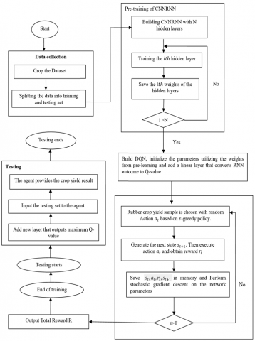
where, $\left(x_{T}\right)$ is a terminal cost; $\left(x_{t}, u_{t}\right)$ is the cost of applying control $u_{t}$ in state $x_{t}$. It is assumed that the initial condition has a Gaussian distribution, with $p\left(x_{0}\right)=\mathcal{N}\left(\mu_{0}, \Sigma_{0}\right)$. The overall flow of the proposed method is illustrated in Figure 3.
The data efficiency is ensured by a model-based $\mathrm{RL}$ technique, in which a framework of the indefinite shift operation $f$ is created to generate open-loop $^{1}$ optimum controllers $u_{0}^{*}, \ldots, u_{T-1}^{*}$ that minimize the value of formula (7). In this way, the learnt framework is modified with the latest understanding, and re-planned after each application of the control series.
Figure 3. Overall flow of CNNRNNDRL
3.8 Long-term estimations
For a specific control series $u_{0}, \ldots, u_{T-1}$, the state distributions $p\left(x_{1}\right), \ldots, p\left(x_{T}\right)$ can be iteratively predicted by:
$p\left(x_{t+1} \mid u_{t}\right)=\iint p\left(x_{t+1} \mid x_{t}, u_{t}\right) p\left(x_{t}\right) p(f) d f d_{x_{t}}$ (9)
For $\mathrm{t}=0, T-1$, a deterministic Gaussian approximation can be made to $p\left(x_{t+1} \mid u_{t}\right)$ through moment matching.
3.9 Expected long-term cost
Adding the estimated immediate expenses to formula (8), the expected long-term cost can be estimated by:
$E\left[l\left(x_{t}, u_{t}\right)\right]=\int l\left(\widetilde{x_{t}}\right) N\left(\widetilde{x_{t}} \mid \widetilde{\mu_{t}}, \widetilde{\Sigma_{t}}\right) \widetilde{d_{x_{t}}}$ (10)
For $t=0, \ldots, T-1, l$ is chosen such that this expectation and the partial derivatives $\partial E\left[\left(x_{t}, u_{t}\right)\right] /$ $\partial x_{t}, \partial E\left[l\left(x_{t}, u_{t}\right)\right] / \partial u_{t}$ can be computed analytically.
$l_{M M}\left(z_{t}, \mathrm{u}_{t}\right)=\mathrm{l}_{\mathrm{MM}}\left(\widetilde{\mathrm{z}_{\mathrm{t}}}\right):=\mathrm{E}\left[\mathrm{l}\left(\mathrm{x}_{\mathrm{t}}, \mathrm{u}_{\mathrm{t}}\right)\right]$ (11)
$\Phi_{\mathrm{MM}}\left(\mathrm{z}_{\mathrm{T}}\right):=\mathrm{E}\left[\Phi\left(\mathrm{x}_{\mathrm{T}}\right)\right]$ (12)
The deterministic mapping (10) projects the mean and covariance of $\widetilde{x}$ into the predicted costs in formula (7). After the CNNRNNDRL is combined with MPC, our method can be denoted by CNNRNNPCDRL, which can forecast rubber yield efficiently with a shorter time series and better classification accuracy.
The proposed CNNRNNPCDRL was compared with various methods, such as DeepLSTM [15], CNNRNN [4], interval deep generative artificial neural network (IDANN) [16], and CNNRNNDRL through rubber yield prediction experiments on the dataset [10]. The performance of each method was measured by precision, recall, and F-measure. The experimental results show that our method achieved a better forecast effect than the contrastive methods from 2018 to 2021, thanks to the use of parameters like soil, rainfall, humidity, temperature, and average wind speed. For experimental purpose, three kernels of the size 4×4 in each convolutional layer. Only 24 outputs were set for the fully connected layer and LSTM layer.
The forecast accuracy was evaluated by comparing the predicted rubber yield with the actual rubber yield in the dataset. The mismatch and match between the two values are defined as:
4.1 Accuracy
The accuracy of each method is defined as the correctly predicted instances as a proportion of all instances:
Accuracy $=\frac{T P+F P}{T P+T N+F P+F N}$
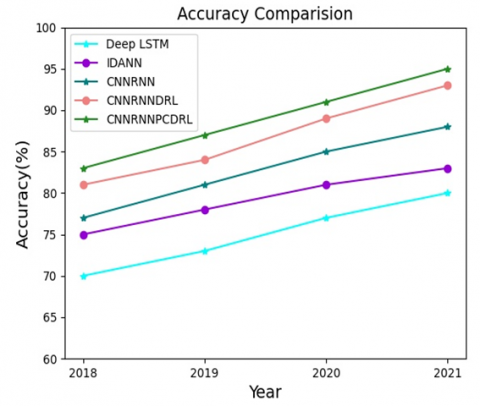
Table 1 and Figure 4 compare the rubber yield prediction accuracies of our method with Deep LTSM, IDANN, CNNRNN, and CNNRNNDRL. The x-axis represents the rubber yield prediction for future years; the y-axis represents the accuracy range.
Table 1. Comparison of accuracy
|
Years |
Methods |
||||
|
Deep LSTM [15] |
ID- ANN [16] |
CNN-RNN [4] |
CNNRNNDRL |
CNNRNNPCDRL |
|
|
2018 |
70 |
75 |
77 |
81 |
83 |
|
2019 |
73 |
78 |
81 |
84 |
87 |
|
2020 |
77 |
81 |
85 |
88 |
91 |
|
2021 |
80 |
83 |
88 |
93 |
95 |
It can be inferred that the accuracy of the CNNRNNDRLMP structure was 18.57%, 19.17%, 18.18%, and 18.75% greater than that of Deep LSTM, 10.66%, 11.54%, 12.35% and 14.16% greater than that of the IDANN, 7.79% 7.41%, 7.06% and 7.95% greater than that of the CNNRNN, and 2.47%, 3.57%, 3.41% and 2.15% greater than that of the CNNRNNDRL in 2018, 2019, 2020 and 2021, respectively. Hence, our CNNRNNPCDRL method outperforms all the other methods in terms of accuracy.
Figure 4. Comparison of accuracy
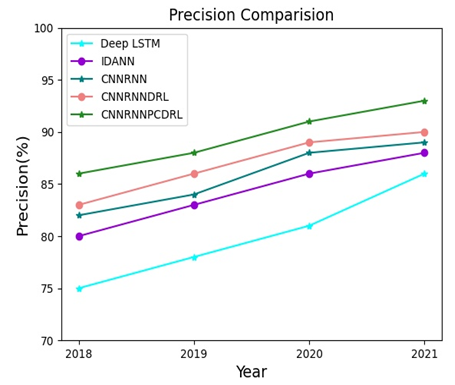
4.2 Precision
Precision measures the ability of a method to forecast the proper rubber yield based on a set of data. It is defined by the percentage of accurately estimated rubber yields at TP and FP rates, or the proportion of actual positives to predicted rubber yields.
precision $=\frac{T P}{T P+F P}$
Table 2 and Figure 5 compare the rubber yield prediction precisions of our method with Deep LTSM, IDANN, CNNRNN, and CNNRNNDRL. The x-axis represents the rubber yield prediction for future years; the y-axis represents the precision range.
Table 2. Comparison of precision
|
Years |
Methods |
||||
|
Deep LSTM |
ID- ANN |
CNN-RNN |
CNNRNNDRL |
CNNRNNPCDRL |
|
|
2018 |
75 |
80 |
82 |
83 |
86 |
|
2019 |
78 |
83 |
84 |
86 |
88 |
|
2020 |
81 |
86 |
88 |
89 |
91 |
|
2021 |
86 |
88 |
89 |
90 |
93 |
It can be inferred that the precision of the CNNRNNPCDRL was 14.67%, 12.82%, 12.34% and 8.14% greater than that of Deep LSTM, 7.5%, 6.02%, 5.81%, and 5.68% greater than that of the IDANN, 4.89%, 4.76%, 3.41%, and 4.49% greater than that of the CNNRNN, and 3.61%, 2.33%, 2.25%, and 3.33% greater than that of the CNNRNNDRL in 2018, 2019, 2020 and 2021, respectively. This means our method achieves better precision than any of the contrastive methods.
Figure 5. Comparison of precision
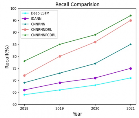
4.3 Recall
Recall assesses the ability of a method to identify each eigenvector of interest in a set of data. It is often depicted as the ratio of accurately predicted rubber yields TP and FN rates, or the proportion of observed positive cases.
Recall $=\frac{T P}{T P+F N}$
Table 3 and Figure 6 compare the rubber yield prediction recalls of our method with Deep LTSM, IDANN, CNNRNN, and CNNRNNDRL. The x-axis represents the rubber yield prediction for future years; the y-axis represents the recall range.
It can be inferred that the recall of the CNNRNNPCDRL was 21.88%, 28.79%, 30.89%, 36.62% greater than that of the Deep LSTM, 18.18%, 23.19%, 25.35%, and 29.33% greater than that of the IDANN, 13.04%, 16.44%, 15.58%, 14.12% greater than that of the CNNRNN, and 8.33%, 6.25%, 3.49%, 2.11% greater than that of the CNNRNNDRL in 2018, 2019, 2020 and 2021, respectively. The comparison shows that our method realizes relatively high recall values, compared to all other existing methods.
Table 3. Comparison of recall
|
Years |
Methods |
||||
|
Deep LSTM |
ID- ANN |
CNN-RNN |
CNNRNNDRL |
CNNRNNPCDRL |
|
|
2018 |
64 |
66 |
69 |
72 |
78 |
|
2019 |
66 |
69 |
73 |
80 |
85 |
|
2020 |
68 |
71 |
77 |
86 |
89 |
|
2021 |
71 |
75 |
85 |
95 |
97 |
Figure 6. Comparison of recall
4.4 F-measure
The approximate prediction of rubber yields can be calculated by the harmonic average of precision and recall, i.e., the F-measure:
F-measure $=\left(\frac{\text { Precision } \cdot \text { Recall }}{\text { Precision }+\text { Recall }}\right) \times 2$
Table 4 and Figure 7 compare the rubber yield prediction F-measures of our method with Deep LTSM, IDANN, CNNRNN, and CNNRNNDRL. The x-axis represents the rubber yield prediction for future years; the y-axis represents the F-measure range.
It can be inferred that the F-measure of the CNNRNNPCDRL was 27.70%, 20.83%, 22.67%, and 20.51% greater than Deep LSTM, 15.28%, 14.47%, 17.95%, and 17.50% greater than that of the IDANN, 10.67%, 11.54%, 12.19%, and 9.30% greater than that of the CNNRNN 5.06%, and 6.09%, 6.97%, and 2.17% greater than that of the CNNRNNDRL in 2018, 2019, 2020 and 2021, respectively. Thus, our method outshines all the contrastive methods with a high F-measure.
Table 4. Comparison of F-measure
|
Years |
Methods |
||||
|
Deep LSTM |
ID- ANN |
CNN-RNN |
CNNRNNDRL |
CNNRNNPCDRL |
|
|
2018 |
65 |
72 |
75 |
79 |
83 |
|
2019 |
72 |
76 |
78 |
82 |
87 |
|
2020 |
75 |
78 |
82 |
86 |
92 |
|
2021 |
78 |
80 |
86 |
92 |
94 |
Figure 7. Comparison of F-measure
This paper proposes an innovative method for rubber yield prediction, denoted as CNNRNNPCDRL, after analyzing various influencing factors, e.g., soil, rainfall, humidity, temperature, and average wind speed. To improve the prediction accuracy, a Q-DRL model was applied using the optimum reward cycles. Then, the rubber yield was predicted with a DQN model built on top of the QL. Based on the input variables, the QL network creates a rubber yield forecast environment. The rubber yield was predicted by the RL agent with a mixture of parameterized attributes along with a threshold. Moreover, the agent accepts an overall rate for the actions executed. If the time series to too long, however, the CNNRNN-based DRL could suffer vanishing gradients. To solve the problem, the CNNRNN-based DRL was coupled with probabilistic predictive modeling strategies to mitigate the uncertainty in statistical predictions. The DRL-based MPC uses GPs to learn a probabilistic transition model, which incorporates system ambiguity and long-term estimations, reducing the negative effect of system failure. Finally, the MPC was adopted to determine the control series that lowers the predicted long-term price. The effectiveness of the proposed method was demonstrated by accuracy, precision, recall, and F-measure.
[1] Rivano, F., Mattos, C.R., Cardoso, S.E., Martinez, M., Cevallos, V., Le Guen, V., Garcia, D. (2013). Breeding Hevea Brasiliensis for yield, growth and SALB resistance for high disease environments. Industrial Crops and Products, 44: 659-670. https://doi.org/10.1016/j.indcrop.2012.09.005
[2] Varghese, L.R., Vanitha, K. (2021). An ontology model to assess the agro-climatic and edaphic feasibility of a location for rubber cultivation. International Journal of Recent Technology and Engineering, 8(3): 1424-1430. https://doi.org/10.35940/ijrte.B3681.098319
[3] Khaki, S., Wang, L. (2019). Crop yield prediction using deep neural networks. Frontiers in Plant Science, 10: 621. https://doi.org/10.3389/fpls.2019.00621
[4] Khaki, S., Wang, L., Archontoulis, S.V. (2020). A CNN-RNN framework for crop yield prediction. Frontiers In Plant Science, 10: 1750. https://doi.org/10.3389/fpls.2019.01750.
[5] Haque, F.F., Abdelgawad, A., Yanambaka, V.P., Yelamarthi, K. (2020). Crop yield prediction using deep neural network. In 2020 IEEE 6th World Forum on Internet of Things (WF-IoT), pp. 1-4. https://doi.org/10.1109/WF-IoT48130.2020.9221298
[6] Kalaiarasi, E., Anbarasi, A. (2021). Crop yield prediction using multi-parametric deep neural networks. Indian Journal of Science and Technology, 14(2): 131-140. https://doi.org/10.17485/IJST/v14i2.2115
[7] Anjula, A., Narsimha, G. (2016). Crop Yield prediction with aid of optimal neural network in spatial data mining: New approaches. International Journal of Information and Computation Technology, 6(1): 25-33.
[8] Qaddoum, K., Hines, E., Iliescu, D. (2012). Yield prediction technique using hybrid adaptive neural genetic network. International Journal of Computational Intelligence and Applications, 11(04): 1250021. https://doi.org/10.1142/S1469026812500216
[9] Bu, F., Wang, X. (2019). A smart agriculture IoT system based on deep reinforcement learning. Future Generation Computer Systems, 99: 500-507. https://doi.org/10.1016/j.future.2019.04.041
[10] India meteorological department of Kerala. http://mausam.imd.gov.in/Thiruvananthapuram.
[11] For the Rubber Research Institute of India (Rubber-board). http://rubsis.rubberboard.org.in/app/index.html?lang=en
[12] Khan, M.A., Peters, S., Sahinel, D., Pozo-Pardo, F.D., Dang, X.T. (2018). Understanding autonomic network management: A look into the past, a solution for the future. Computer Communications, 122: 93-117. https://doi.org/10.1016/j.comcom.2018.01.014
[13] Littman, M.L. (2001). Value-function reinforcement learning in Markov games. Cognitive Systems Research, 2(1): 55-66. https://doi.org/10.1016/S1389-0417(01)00015-8
[14] Kamthe, S., Deisenroth, M. (2018). Data-efficient reinforcement learning with probabilistic model predictive control. In International Conference on Artificial Intelligence and Statistics, pp. 1701-1710. https://arxiv.org/abs/1706.06491.
[15] Sharma, S., Rai, S., Krishnan, N.C. (2020). Wheat Crop Yield Prediction Using Deep LSTM Model. arXiv print. https://arxiv.org/abs/2011.01498.
[16] Elavarasan, D., Vincent, P.D. (2020). Crop yield prediction using deep reinforcement learning model for sustainable agrarian applications. IEEE Access, 8: 86886-86901. https://doi.org/10.1109/ACCESS.2020.2992480