Venkata Rao Maddumala* | Arunkumar R
© 2021 IIETA. This article is published by IIETA and is licensed under the CC BY 4.0 license (http://creativecommons.org/licenses/by/4.0/).
OPEN ACCESS
This paper presents a novel method for body mass index prediction and classification based on the multinomial logistic regression model. The facial geometrical features are extracted and the logistic regression model parameters estimated based on the features. Based on the model parameters, the logistic model is fit in to predict the body mass index and classifies. Two different facial datasets are taken into account for the experiments. Each dataset is divided into two sets. One set is used to estimate the parameters while the other is used to fit-in the model and predicts the body mass index and classifies itself. The obtained outcome results show that the performance of the proposed method is comparable to the state-of-the-art techniques.
body mass index, prediction, classification, multinomial logistic regression, morphological facial cues
The face is the mirror of the mind, and eyes without speaking confess the secrets of the heart.
― Saint Jerome
As the above proverb states, one can determine, describe, and judge a person based on the facial expression which exposes the person’s feeling or situation; the feeling or situation might be happy or sad or physical illness, in general, whatever it is. The literature reveals that one can observe much information about a person from the face of that person. Pharm et al. [1] have suggested, for centuries, that the human face reflects the attributes of gender, ethnicity, attractiveness, emotions, personality traits and so on has been the subject of speculation. The literature reports that the facial attractiveness is attributed to longevity [2], reproductive health [3, 4] and some physical illness symptoms like cold, nausea, backache, etc. [5], heterozygous human leukocyte antigen (HLA) genes [6]. De Jager et al. [7] have reported that Facial adiposity is strongly regressed to attractiveness and health, with more massive faces are judged to be more unattractive and unhealthier. The facial adiposity has also correlated with many actual health outcomes including, such as cold and flu number, duration of colds and flu, frequency of antibiotic use, respiratory illness, blood pressure, cardiovascular illness, salivary progesterone, psychological well-being, arthritis, diabetes, circulating testosterone, immune function, and oxidative stress. A recent study has demonstrated that the facial adiposity, the perception of weight in the face, is associated with perceived health and attractiveness in a nonlinear relationship, whereas the facial adiposity and blood pressure is linearly correlated. It is observed from the literature that one can obtain many of information about a person, based on the facial cues, which are related to health, cognizant, societal, psychological, ethnicity and so on. Although several approaches have been developed to address the above problems, still, there exists a lacking in measuring the facial structure and the deployment of the classification techniques. The physical structure and shape of the face have to be precisely predicted, then only it leads to good results, because whatever it may be, the Body Mass Index (BMI), health condition, heterozygous human leukocyte antigen and other matters, which rely on the measurement of the face.
Coetzee et al. [8] proposed three geometrical facial cues, such as width-to-height ratio (WHR), cheek-to-jaw-width ratio (CJWR), and perimeter to area ratio (PAR), to assess the association between the facial cues and the BMI. They have deployed the statistical methods, namely Skewness, kurtosis, and Pearson’s correlation coefficient, to assess the association between the facial cues and the BMI; reported that the WHR, CJWR, and PAR are closely associated with BMI of both Caucasian and African faces of male while the WHR and CJRW correlated with BMI of the female. Subsequently, Pham et al. [1] have conducted a study on Sasang facial typology. In which, they have introduced the facial masculinity indexes, in addition to the geometrical cues; they have applied Pearson’s correlation coefficient to assess the degree of association of the facial cues with the BMI and used One-way ANOVA to measure the difference between the groups; further they have employed the logistic regression model to predict the association between the facial cues and the BMI. Finally, they report that the PAR, WHR, CJWR and eye size (ES) highly correlated with BMI; they have also suggested that BMI and CJWR can be used to discriminate the TaeEum (TE) type from the SoYang (SY) and SoEum (SE) types in Sasang typing. Wen and Guo [9] have proposed an automated computational system, based on the regression analyses with different methods, which predicts the BMI from geometrical facial cues. They have introduced a three more new features: the lower face to face height ratio (LF/FH), face width to lower face height ratio (FW/LFH) and mean of eyebrow height (MEH), in addition to the features. They have reported that the proposed system shows a good association between the geometrical cues and the predicted BMI. Wolffhechel et al. [10] have used principal component analysis (PCA) for predicting the BMI from facial cues. Mayer et al. [11] have measured the relationship between the BMI and the waist-to-hip-ratio (WHR) with facial shape and colour features. They have applied multivariate linear regression to estimate the association between facial shape and texture with BMIand WHR. Barr et al. [12] have attempted to examine whether the existing methods correctly identifies the facial cues and BMI. To arrive the above objective, they have deployed the regression to assess the relationship between the facial cues and BMI; further, they have used the Correlation and Contingency table analyses and reported that facial image features are a viable measure for the dissemination of human research related to facial cues and BMI, although, they suggested that it requires further analysis.
The statistical models, such as Linear Regression, Non-linear regression, Logistics regression, PCA, and Pearson's correlation, have been deployed in previous studies that are more appropriate for two classes of data classification problems than the data that has more than two categories of responses. In the case of BMI categorization, there are four different classes, as demonstrated in Table 1. Thus, this paper believes that the multinomial logistic regression is the most appropriate for identifying the association of BMI with geometrical facial cues and the BMI categorization. Also, the aforementioned geometrical features could be more useful for predicting the BMI but not for age, ethnicity, race, gender. The facial characteristics and BMI are influenced by age and gender [13]. If the colour feature and texture feature (facial skin surface) incorporated into the above geometrical features it could result in more information like BMI, age, gender, ethnicity, and race; these features are also could be more useful for face recognition. The BMI is calculated by the traditional method [14] as given below, based on an individual's height and weight.
$B M I=\left\{\begin{array}{l}\frac{\text { weight }(\mathrm{kg})}{\text { height }(\mathrm{m})^{2}} \\ \text { or } \\ \frac{\text { weight }(\mathrm{lb}) \times 0.703}{\text { height }(\text { inch })^{2}}\end{array}\right.$
Table 1. BMI categories and BMI range
|
Category |
BMI range |
|
Underweight |
<18.5 |
|
Normal |
18.5 to 24.9 |
|
Overweight |
25.0 to 29.9 |
|
Obese |
>30 |
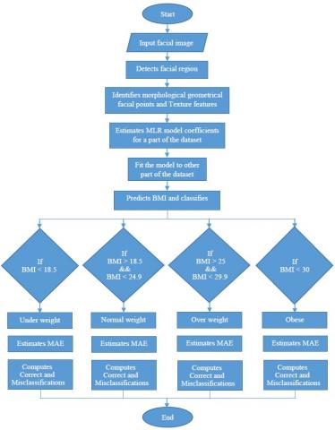
Figure 1. Outline of the proposed method
In this study, we consider the MORPH-II facial image dataset designed for the academic purpose, which contains about 55,000 images with different categories. Different kinds of features, such as geometrical features, colour, and texture features, are extracted; further, these features used for predicting BMI, age, gender, ethnicity, race, etc. Also, the predicted features can be used for other purposes like face recognition, health care and so on. The study involves in voluminous of image data and different categories of data (structured and unstructured), which leads to Big data analytics or Big data environment. These factors motivated us to develop a new method, based on the Multinomial Logistic Regression (MLR) for prediction of BMI and its categorization as well as classification of other features, which extracts multifaceted features and that can be used for other purposes.
The literature shows that colour features have been used rarely to predict the BMI [10, 11], Wolffhechel et al. have extracted colour feature based on the PCA model, and used to predict the BMI. The literature reveals that almost all the research works used geometrical features for the prediction of BMI, age, gender, race, etc., not the colour or texture features of the face. As suggested above, the colour feature and texture feature will result in a promising outcome that not only related to the prediction of the BMI but also the age, gender, race and so on. Thus, this paper extracts seven geometrical features: CWJWR, CWUFHR, PAR, ASoE, FHLFHR, FWLFHR, MEH, and texture feature; and employs the MLR model to predict the association of the facial cues with the BMI and other matters.
Outline of the proposed method
It can be shown from Figure 1 that order to predict the BMI of an individual, two different datasets, such as MORPH-II and VIP_Attribute, considered for the experiments; each dataset was divided into two sets of facial images, viz. Set-1 and Set-2. The facial images of each set were randomly selected using the stratified random sampling technique because the original datasets comprise different categories of facial images. The MLR model coefficients are estimated from the images in Set-1. The model coefficients are estimated by the LASSO method. Based on the estimated coefficients, the MLR model is fitted to each facial image of the Set-2, and the BMI is predicted; and classified into any one of the four categories of BMI. The MAE is computed between the observed and estimated BMI of each subject of the Set-2. Similarly, the model coefficients are estimated to the facial images of the Set-1, and BMI is predicted for each subject of Set-1. The same BMI prediction process is performed for the VIP_Attribute dataset also. The overall process of the proposed method has been outlined in the following flow diagram.
3.1 Model formulation
The given face image converted to the YCbCr colour model for the computational simplicity, where Y represents the luminance, i.e., intensity (brightness) values of the face image; the Cb and Cr represent the blue-difference and the red-difference Chroma components, respectively. In this study, the facial cues such as seven morphological features and texture feature are extracted from each face image. The facial fiducial cues comprise Cheekbone width to Jaw width ratio (CWJWR), Cheekbone width to Upper Facial Height Ratio (CWUFHR), Perimeter to Area of the polygon (PAR), Average Size of Eyes (ASoE), Face Height to Lower Face Height Ratio (FHLFHR), Face width to Lower Face Height Ratio (FWLFHR), and Mean of Eyebrow Height (MEH); colour feature and the texture feature. The geometrical cues and the texture feature are extracted from the grayscale image. Let the eight features be assumed as independent and identically distributed to a multinomial random process. The probability mass function of the above process with mean nρiand variance nρi(1-ρi) can be defined as follows.
$F\left(S F_{1}, \ldots, S F_{9} ; p_{1}, \ldots p_{9}\right)$
$=\left\{\begin{array}{ll}\frac{n !}{S F_{1} !, \ldots, S F_{9} !} p_{1}^{S F_{1}} \times \ldots \times p_{9}^{S F_{9}}, & \text { when } \sum_{i=1}^{9} S F_{i}=n \\ 0, & \text { otherwise, }\end{array}\right.$ (1)
where, n is the number of subjects (samples = number of face images); $S F_{(.)}$ is the salient features of the face image; $S F_{i}=\left\{\begin{array}{l}\text { CWJWR, CWUFHR, PAR, ASoE, FHLFHR, } \\ \text { FWLFHR, } M E H, T F\end{array}\right\}$; $p_{(\cdot)}$ is the feature probabilities.
In order to achieve the objective of this study, viz. predicting the BMI of an individual from the salient facial features. The BMI is treated as a response variable with four categories as depicted in Eq. (2) whereas the face cues are regarded as the independent variables. As the dependent variable, BMI has four categories; it is appropriate to build an MLR model with nine explanatory variables. The proposed MLR model is expressed in Eq. (2).
$B M I_{k, i}=\lambda_{0, k}+\lambda_{1, k} S F_{1, i}+\lambda_{2, k} S F_{2, i}+\ldots+\lambda_{10, k} S F_{10, i}$ (2)
where, BMIk,i denotes the k-th category $\left(\right. s.t. k=\left\{\begin{array}{l}\text { UW: underweight; NW: normal weight ; } \\ \text { OW:overweight ; OB: obese }\end{array}\right\})$ of i-th subject (face); λ10,krepresents the regression coefficient of the Cr (9-th facial feature of SF) feature and k-th category.
The Eq. (2) can be written in an expanded form as follows.
$\left.\begin{array}{l}U W i=\lambda_{0, k}+\lambda_{1, U W} S F_{1, i}+\lambda_{2, U W} S F_{2, i}+\ldots+\lambda_{10, U W} S F_{10, i} \\ N W i=\lambda_{0, k}+\lambda_{1, N W} S F_{1, i}+\lambda_{2, N W} S F_{2, i}+\ldots+\lambda_{10, N W} S F_{10, i} \\ O W i=\lambda_{0, k}+\lambda_{1, W W} S F_{1, i}+\lambda_{2, O W} S F_{2, i}+\ldots+\lambda_{10, O W} S F_{10, i} \\ O B i=\lambda_{0, k}+\lambda_{I, O B} S F_{1, i}+\lambda_{2, O B} S F_{2, i}+\ldots+\lambda_{10, O B} S F_{10, i}\end{array}\right\}$ (3)
The above equation can be written in a compact form as given in Eq. (4).
$B M I_{k, i}=\lambda_{k} \cdot S F_{i}$ (4)
where, BMI is a column vector; λk is a set of regression coefficients that are associated with the outcome, k; SFi is a set of explanatory variables that are associated with observation, i.
3.1.1 Estimate of regression coefficients
To estimate the coefficient of the proposed MLR model, the Least Absolute Shrinkage and Selection Operator (LASSO) is used, which is introduced in ref. [15]. A multinomial logistic model fitting can be performed in straightforward using LASSO, which yields better or similar estimates than the Maximum Likelihood and Ordinary Least Square Estimator [15, 16]. Thus, this paper makes use of the LASSO to estimate the coefficients of the proposed MLR model. The model coefficients are estimated as follows.
$\hat{\lambda}^{L}=\arg \min \sum_{i=1}^{n}\left(B M I_{i}-\lambda_{0}-\sum_{j=1}^{k} \lambda_{j} S F_{i, j}\right)^{2}$ (5)
$\hat{\lambda}^{L}=\arg \min \sum_{i=1}^{n} \frac{1}{2}\left(B M I_{i}-\lambda_{0}-\sum_{j=1}^{k} \lambda_{j} S F_{i, j}\right)^{2}+\gamma \sum_{\mathrm{j}=1}^{\mathrm{k}}\left|\hat{\lambda}_{\mathrm{j}^L}\right|$ (6)
with the constraint, $\sum_{j=1}^{k}\left|\hat{\lambda}_{j}^L\right| \leq t, \quad \gamma=\frac{1}{\sum_{j=1}^{k}\left|\hat{\lambda}_{j}^L\right|}$.
The LASSO forward algorithm starts with all coefficients, $\hat{\lambda}$, equal to zero; finds the predictor SFj, which is most correlated to BMI, and incorporates it into the model; computes the residuals $r=B M I_{k}-B \hat{M} I_{k}$ at each stage, and adds to the model predictor that most correlated with r; continue still, finally all predictors are incorporated in the model. The LASSO for a multinomial logit model is expressed in Eq. (4).
$\hat{\lambda}^{L}=\arg \max \left[l(\hat{\lambda})-\gamma \sum_{i=}^{L} \sum_{j=1}^{k}\left|\hat{\lambda}_{j}^{L}\right|\right]$ (7)
where, $l(\hat{\lambda})$ is the estimate of the log-likelihood function. The log-likelihood of λ is expressed in Eq. (8).
$l(\lambda)=\sum_{i=1}^{n} \sum_{j=1}^{k}\left[B M I_{j, i} g_{j}\left(S F_{i}\right)-\ln \left(1+e^{g_{j}\left(S F_{i}\right)}\right)\right]$ (8)
The MLR model can be written in the form of the logit equation as in Eq. (9). It is the natural logarithm of the odds, viz. the ratio of the probability of a level and the reference. Here, the Normal Weight (NW) is considered as the reference/control level of the categorical response variable, BMI.
$g_{k}(S F)=\ln \left\{\frac{\operatorname{Pr}(Y=k \mid S F)}{\operatorname{Pr}(Y=N W \mid S F)}\right\}=\lambda_{0,1}+\sum_{i=1}^{10} \lambda_{i, 1} S F_{i}$; (9)
s.t. $k=[U W, O W, O B]$
The above expression can be compactly written in matrix form as in Eqns. (3) and (4) without the latent variable, λ0,1.
4.1 Experimental setups
In order to validate the proposed prediction method, the height, weight, and BMI predicted from the facial cues extracted from the following datasets, such as MORPH-II (MORPHology) [17] and VIP_attributedataset(Very Important Person_attribute dataset) [18]. The following subsections discuss the structure of the datasets and feature extraction methods.
4.1.1 Face image datasets
MORPH-II: The MORPH-II is a longitudinal face database developed for researchers investigating all facets of adult age-progression, e.g. face modelling, photo-realistic animation, face recognition, etc. The MORPH-II academic version dataset was purchased on our interest at the rate of \$ 99 for our research use. The details of the dataset [19] are presented in Table 2. Further, a set of 29,168 face images sampled, based on stratified random sampling method, from the dataset, which is divided into two sets, such as Set-1 (S1) and Set-2 (S2). Some of them classified into six groups in terms of age, viz. people below 20 years grouped into Age group 1; between 19 and 30 to Age group 2; between 29 and 40 to Age group 3; between 39 and 50 to Age group 4; between 49 and 60 to Age group 5; people above 60 years into Age group 6. The MORPH-II dataset comprised of five categories, such as Black, White, Asian, Hispanic, Others, in terms of race and geographical regions. The VIP_Attribute dataset also has two categories: male and female. Thus, the stratified random sampling techniques was adopted to select the sample images from each category. The details of the two subsets have been given in Table 3.
Table 2. MORPH-II facial images
|
|
Black |
White |
Asian |
Hispanic |
Other |
Total |
|
Male |
36,821 |
7,958 |
140 |
1,661 |
64 |
46,644 |
|
Female |
5,756 |
2,590 |
13 |
99 |
32 |
8,490 |
|
Total |
42,577 |
10,548 |
153 |
1,760 |
96 |
55,134 |
Table 3. Subsets of the MORPH-II facial images
|
Subclasses |
Set-1 |
Set-2 |
|
Black female |
908 |
902 |
|
Black male |
2642 |
2692 |
|
White female |
1006 |
1022 |
|
White male |
2717 |
2707 |
|
Age group 1 |
3679 |
3685 |
|
Age group 2 |
3144 |
3152 |
|
Age group 3 |
437 |
475 |
|
Total |
14533 |
14635 |
Table 4. Subsets of the male and female groups
|
Subclasses |
Set-1 |
Set-2 |
|
Female |
313 |
200 |
|
Male |
313 |
200 |
|
Total |
626 |
400 |
VIP_Attribute dataset: The VIP_attribute dataset is freely available benchmark dataset, which is composed of 1026 subjects, of which, 513 female and 513 male face images of the celebrities. It is exclusively designed for studying the BMI, height, and weight of a subject based on the facial images, which is collected from Dantcheva et al. [18]. It was further divided into two sets of male and female groups as given Table 4. The MLR model coefficients are estimated based on the facial images of Set-1; based on the estimated coefficients, the model is fitted to the facial images of Set-2, and the BMI values are predicted based on the facial cues.
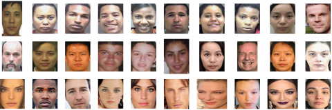
Figure 2. Cropped face images. rows 1 and 2: MORPH-II face images; row 3: VIP_Attribute dataset
As the above datasets were exclusively designed for the experimental purpose of the study relating to prediction of the height, weight, and BMI of a subject from the facial cues, they do not require any pre-process except cropping the facial region. Hence, this paper extracts the facial features, such as geometrical features, texture feature, and colour feature, in straightaway. The cropped facial image regions, for a sample, of the MORPH-II and VIP_Attribute datasets have been presented in Figure 2.
4.1.2 Feature extraction
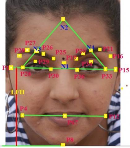
The hierarchical Hetero-PSO-Adaboost-SVM face detector [20] method proposed was adopted here to detect the face-region, i.e., the region of interest (RoI). After detecting the face-region, the Active Shape Model (ASM) is applied, which marks/identifies the facial fiducial points that are very useful to predict the BMI. Mainly seven salient geometrical cues are computed, based on facial fiducial points demonstrated in Figure 3, which are described below.
Figure 3. Geometrical facial fiducial points
CWJWR (Cheekbone width to Jaw width ratio) feature: represents the ratio of the cheekbone width to Jaw width, which is defined in Eq. (10).
$C W J W R=\frac{|P 15-P 1|}{|P 12-P 4|}$ (10)
where, │P12-P4│ represents the Cheekbone width while │P15-P1│ means the Jaw width.
CWUFHR (Cheekbone width to Upper Facial Height Ratio): represents the ratio of the Cheekbone Width to Upper Facial Height, which is presented below.
$C W U F H R=\frac{|P 12-P 4|}{|N 2-P 67|}$ (11)
where, │P12-P4│ denotes the Cheekbone width; │N2-67│denotes Upper Facial Height.
PAR (Perimeter to Area of polygon): defines the ratio of perimeter to area of the polygon, which is computed by,
$P A R=\frac{\text { Perimeter }(P 1 P 4 P 8 P 12 P 15 P 1)}{\text { Area }(P 1 P 4 P 8 P 12 P 15 P 1)}$ (12)
ASoE (Average Size of Eyes): represents the average size of both eyes with respect to horizontal distance, which is derived by,
$A S o E=\frac{1}{2}(|P 33-P 28|-|P 35-P 30|)$ (13)
FHLFHR (Face Height to Lower Face Height Ratio):
$F H L F H R=\frac{|L F H|}{|N 2-P 8|}$ (14)
where, LFH is the lower face height, which means the distance between the Cheekbone and the lowest point in the Jaw that illustrated in Figure 3; │N2-P8│represents the distance between the topmost point of the forehead (N2) and the lowest point of the Chin (P8).
FWLFHR (Face width to Lower Face Height Ratio): represents the ratio face width to lower face height, which is defined as:
$F W L F H R=\frac{|P 15-P 1|}{|L F H|}$ (15)
MEH (Mean of Eyebrow Height): represents the mean height of the eyes, which is computed by the expression given in Eq. (16).
$M E H=\frac{1}{6}\left(\begin{array}{l}{[P 22-P 28]+[N 30-P 29]+[P 25-P 30]+} \\ {[P 19-P 35]+[N 4-P 34]+[P 16-P 33]}\end{array}\right)$ (16)
Texture features: It characterizes the facial-skin surface, by which one can predict the attributes like age, gender, and race. This paper deploys the Autocorrelation Coefficient (γ) to characterize the texture properties of the facial-skin surface. The autocorrelation is computed on the specific region of interest, such as forehead, chin, cheeks, using the function expressed in Eq. (17). The ACC is computed as follows.
$\gamma_{k}=\frac{\sum_{i=1}^{n}\left(f_{i}-\bar{f}\right)\left(f_{i-k}-\bar{f}\right)}{\sum_{i=1}^{n}\left(f_{i}-\bar{f}\right)^{2}}$ (17)
where, $\overline{\mathrm{f}}=\frac{1}{\mathrm{n}} \sum_{\mathrm{i}=1}^{\mathrm{n}} \mathrm{f}_{\mathrm{i}}$.
The numerator in Eq. (17) represents the covariance of the pixels in the region while the denominator represents variance; $\bar{f}$ represents the mean value of the pixels in the region.
This paper categorizes the computed ACC into three class, such as class 1 (C1), class (C2), and class 3 (C3). The ACC value falls in the interval 0 to 0.4 categorized into C1, which represents the people in the age group of less than 30 years; the ACC value falls in the interval 0.4 to 0.7 categorized into C2, which means the people in the age in between 31 to 60 years; the ACC value falls in the interval 0.7 to 1.0 categorized into C3 that represents the age people in the age group greater than 60 years.
Feature vector database: The extracted features formulated to a feature vector matrix, which consists of 29,168 rows and 8 columns; each column represents an attribute of the facial image, and each row means a subject.
4.2 Measure of performance
Mean Absolute Error (MAE) was deployed to validate and verify the performance of the proposed method. The MAE was computed using the expression given in Eq. (18).
$M A E=\frac{1}{n} \sum_{i=1}^{n}\left|b_{i}-\hat{b}_{\mathrm{i}}\right|$ (18)
where, bi and $\hat{{b}_{\mathrm{i}}}$ represent the observed and predicted BMI of i-th subject.
In order to empirically validate the proposed method, which implemented with the above datasets using Python cv2 with the system specification: Intel Core i5 processor-based PC with 3 GHz, 8 GB DDR4 RAM, Intel Mother Board D97, and 4.0 GB Video Card.
This paper is not concentrating more on establishing the relationship between the facial fiducial points and BMI. Because the previous studies [1, 8, 9, 12, 21] proved the existence of the relationship between the facial cues and the BMI; instead, this paper straight away goes to the prediction of BMI [22], by which, it convinces the objective of the study that the MLR model yields better results than the other methods. Hence, the facial features, such as geometrical and texture, extracted from each facial image [23, 24] were straight away subject to the experiments using the MLR model discussed in Section 3. First, the MLR model coefficients were estimated, based on the LASSO estimator discussed in Section 3.1.1, for the facial images of all categories of both Sets and the combined images, i.e. for all 29,168 images. The model fitted to all groups of images in Set-2, and the predicted BMI values were obtained. The MAE and the classification rate, for the BMI predicted by the MLR model, were computed for all the categories of subclasses of Set-2 of the MORPH-II facial dataset.
The proposed method results in average MAE rate of 3.81 for the Black female subject and 3.54 for Black male. An average MAE rate of 3.25 for White female and 3.16 for White male. Besides, the average MAE rate calculated for age-group-wise that results in an average rate of 3.84 for Age group-1; 3.05 for Age group-2; 3.85 for Age group-3.as shown in Figure 4.
Also, an average classification rate calculated, which gives 92.55% correct classification and 10.38% misclassification for the Black female category. A 93.08% correct classification and 6.92% misclassification rate for Black male; 92.55% correct classification and 7.45% misclassification rate for White female; 96.23% correct classification and 3.78% misclassification rate for White male. Moreover, the average rate of correct classification of 92.15% and 3.60% misclassification obtained for the people in the Age group-1. A 91.19% correct classification and 8.83% misclassification rate achieved for Age group-2. 92.89% correct classification and 8.61% misclassification rate for Age group-3. The computed MAE and the classification rates have been presented in Table 5. A Bar chart was drawn for the average values of the MAE obtained between the observed and predicted BMIs for the MORPH-II dataset that has been depicted in Figure 4. Also, a Bar chart was drawn for the average of the classification and misclassification rates computed for the predicted BMIs, which has been demonstrated in Figure 5.
The performance of the proposed method was compared to [9] in terms of MAE. The comparative study shows that the proposed method yields better results than the existing methods. Besides, the predicted BMIs were classified, which demonstrates that the proposed method predicts more precisely than the state-of-the-art method.
Furthermore, the MLR coefficients estimated, based on the facial images of Set-1 of the VIP_Attribute dataset. The estimated coefficients used to predict BMI of facial images in the Set-2 and the obtained results have been presented in Table 6.
Figure 4. Average values of MAE between observed and predicted BMIs
Figure 5. Average values of correct classification and misclassification rates for MORPH-II dataset
Table 5. Category-wise MAE and classification rate (%) for subclasses of Set-2 for MORPH-II facial dataset. The value within the parenthesis means the misclassification rate
|
Subclasses |
BMI Category |
MAE |
Classification rate (%) |
|
Black female |
Underweight |
3.91 |
89.62 (10.38) |
|
Normal |
2.96 |
93.59 (06.41) |
|
|
Overweight |
4.12 |
91.14 (08.86) |
|
|
Obese |
4.26 |
95.86 (04.14) |
|
|
Black male |
Underweight |
3.28 |
90.25 (09.75) |
|
Normal |
2.62 |
94.81 (05.19) |
|
|
Overweight |
3.94 |
91.89 (08.11) |
|
|
Obese |
4.31 |
95.37 (04.63) |
|
|
White female |
Underweight |
3.53 |
89.06 (10.94) |
|
Normal |
2.41 |
96.08 (03.92) |
|
|
Overweight |
2.93 |
90.18 (09.82) |
|
|
Obese |
4.15 |
94.86 (05.14) |
|
|
White male |
Underweight |
3.36 |
96.27 (03.73) |
|
Normal |
2.21 |
96.28 (03.72) |
|
|
Overweight |
2.69 |
95.98 (04.02) |
|
|
Obese |
4.38 |
96.37 (03.63) |
|
|
Age group-1 |
Underweight |
3.68 |
89.41 (10.59) |
|
Normal |
3.93 |
91.59 (08.41) |
|
|
Overweight |
3.24 |
92.82 (07.18) |
|
|
Obese |
4.49 |
94.78 (05.22) |
|
|
Age group-2 |
Underweight |
3.04 |
90.53 (09.47) |
|
Normal |
2.94 |
89.74 (10.26) |
|
|
Overweight |
2.86 |
91.41 (08.59) |
|
|
Obese |
3.38 |
93.08 (06.98) |
|
|
Age group-3 |
Underweight |
4.65 |
90.86 (09.14) |
|
Normal |
3.91 |
91.79 (08.21) |
|
|
Overweight |
3.69 |
92.83 (07.17) |
|
|
Obese |
3.16 |
90.08 (09.92) |
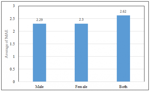
The results presented in Table 6 shows that the proposed MLR method yields 2.29 average MAE rate for male facial images while 2.30 average rate for female; and results in 2.62 MAE average rate for overall facial images as shown in Figure 6. Also, it gives 96.22% average correct classification and 3.78% misclassification for male facial images; 95.55% correct classification and 7.45% misclassification for female; 96.22% correct classification and 3.78% misclassification for overall facial images of the VIP_Attribute dataset. A Bar diagram drawn for the average values of MAE computed between the observed and predicted BMIs, and it has been shown in Figure 6. Moreover, a Bar chart was drawn for the average of the classification and misclassification rates computed for the predicted BMIs, which has been illustrated in Figure 7. The obtained MAE results were compared to the results obtained in which shows that the proposed method outperforms the existing methods.
Table 6. VIP_Attribute dataset. MAE and classification rate for BMI Category-wise
|
Subclasses |
BMI Category |
MAE |
Classification rate |
|
Male |
Underweight |
2.30 |
96.82 (03.18) |
|
Normal |
2.26 |
96.19 (03.81) |
|
|
Overweight |
2.38 |
94.64 (05.36) |
|
|
Obese |
2.20 |
97.24 (02.76) |
|
|
Female |
Underweight |
2.05 |
89.62 (10.38) |
|
Normal |
2.56 |
93.59 (06.41) |
|
|
Overweight |
2.12 |
91.14 (08.86) |
|
|
Obese |
2.46 |
95.86 (04.14) |
|
|
BothMale andFemale |
Underweight |
2.91 |
96.63 (03.37) |
|
Normal |
2.26 |
94.29 (05.71) |
|
|
Overweight |
2.29 |
96.54 (03.46) |
|
|
Obese |
3.01 |
97.43 (02.57) |
Figure 6. Average values of the MAE between the observed and predicted BMIs for VIP_Attribute dataset
Figure 7. Average values of correct classification and misclassification for VIP_Attribute dataset
Two different datasets were subjected to the experiments, which comprise different categories of facial images. Each category of both datasets divided into two sets, i.e., Set-1 and Set-2. The MLR model coefficients estimated, based on LASSO, from both sets. The model fitted to facial images of the Set-2, based on the coefficients estimated from Set-1, to predict the BMI; the predicted BMI automatically classified into any one of the categories of the BMI. The MAE deployed to validate the predicted BMI, and the BMIs were classified into correct classification and misclassification. The MORPH-II dataset gives an average correct classification of 92.86% Black race, whereas it offers 7.18% misclassification; a 94.39% correct classification and 5.62% misclassification for the white race. Also, it results in correct classification up to 92.16% and misclassification up to 8.42% for overall the three age groups. Besides an MAE was calculated, which yields 3.68% for the Black race, whereas it gives 3.21% MAE for White race, and it provides an average of the MAE up to 3.38 for overall age groups of the MORPH-II dataset.
The average MAE was calculated for the VIP_Attribute dataset, which gives up to 2.29 for male facial images, whereas it gives 2.30 for female facial images. Furthermore, the average classification rates calculated, it yields up to 96.22% correct classification whereas 3.78% misclassification for male facial images; it shows up to 92.55% correct classification for female facial images while it turned up to 7.45% misclassification. In overall, the obtained results show that the proposed MLR-based method outperforms the state-of-the-art methods in terms of MAE and classification rates.
The proposed MLR-based method, in future, can be extended with deep learning concepts like the deep convolutional neural network in the domain of face recognition and big data analytics. It can also be deployed for analysing demographical data that pertains to the big-data analytics, such as socio-economic status of the people in a country and impact of the COVID-19 on various sectors like IT industries, Airlines, tourism and so on across the world. We, also, have planned to incorporate colour features and extend for facial recognition, and BMI with other features, such as age, gender, and race.
The authors thank the anonymous reviewers for their valuable suggestions to enhance the quality and the readability of the paper.
[1] Pham, D.D., Do, J.H., Ku, B., Lee, H.J., Kim, H., Kim, Y.J. (2011). Body mass index and facial cues in Sasang typology for young and elderly persons. Evidence-Based Complementary and Alternative Medicine, 2011: 1-9. https://doi.org/10.1155/2011/749209
[2] Henderson, J.J.A., Anglin, J.M. (2003). Facial attractiveness predicts longevity. Evolution and Human Behavior, 24(5): 351-356. https://doi.org/10.1016/S1090-5138(03)00036-9
[3] Soler, C., Núñez, M., Gutiérrez, R., Núñez, J., Medina, P., Sancho, M., Álvarez, J., Núñez, A. (2003). Facial attractiveness in men provides clues to semen quality. Evolution and Human Behavior, 24(3): 199-207. https://doi.org/10.1016/S1090-5138(03)00013-8
[4] Smith, M.J., Perrett, D.I., Jones, B.C., Cornwell, R.E., Moore, F.R., Feinberg, D.R., Boothroyd, L.G., Durrani, S.J., Stirrat, M.R., Whiten, S., Pitman, R.M., Hillier, S.G. (2006). Facial appearance is a cue to oestrogen levels in women. Proceedings of the Royal Society B, 273(1583): 135-140. https://doi.org/10.1098/rspb.2005.3296
[5] Shackelford, T.K., Larsen, R.J. (1999). Facial attractiveness and physical health. Evolution and Human Behavior, 20(1): 71-76. https://doi.org/10.1016/S1090-5138(98)00036-1
[6] Roberts, S.C., Little, A.C., Gosling, L.M., Perrett, D.I., Carter, V., Jonese, B.C., Penton-Voak, I., Petrie, M. (2005). MHC-heterozygosity and human facial attractiveness. Evolution and Human Behavior, 26(3): 213-226. https://doi.org/10.1016/j.evolhumbehav.2004.09.002
[7] De Jager, S., Coetzee, N., Coetzee, V. (2018). Facial adiposity, attractiveness, and health: A review. Front Psychol., 9: 2562: 1-18. https://doi.org/10.3389/fpsyg.2018.02562
[8] Coetzee, V., Chen, J., Perrett, D.I., Stephen, I.D. (2010). Deciphering faces: Quantifiable visual cues to weight. Perception, 39(1): 51-61. https://doi.org/10.1068/p6560
[9] Wen, L., Guo, G. (2013). A computational approach to body mass index prediction from face images. Image and Vision Computing, 31(5): 392-400. https://doi.org/10.1016/j.imavis.2013.03.001
[10] Wolffhechel, K., Hahn, A.C., Jarmer, H., Fisher, C.I., Jones, B.C., DeBruine, L.M. (2015). Testing the utility of a data-driven approach for assessing BMI from face images. PLoS One, 10(10): e0140347. https://doi.org/10.1371/journal.pone.0140347
[11] Mayer, C., Windhager, S., Schaefer, K., Mitteroecker, P. (2017). BMI and WHR are reflected in female facial shape and texture: A geometric morphometric image analysis. PLoS One, 12(1): e0169336. https://doi.org/10.1371/journal.pone.0169336
[12] Barr, M.L., Guo, G., Colby, S.E., Olfert, M.D. (2018). Detecting body mass index from a facial photograph in lifestyle intervention. Technologies, 6(83): 1-8. https://doi.org/10.3390/technologies6030083
[13] Ferrario, V.F., Sforza, C. (1997). Size and shape of soft-tissue facial profile: Effects of age, gender, and skeletal class. The Cleft Palate-Craniofacial Journal, 34(6): 498-504. https://doi.org/10.1597/1545-1569_1997_034_0498_sasost_2.3.co_2
[14] Keys, A., Fidanza, F., Karvonen, M.J., Kimura, N., Taylor, H.L. (1972). Indices of relative weight and obesity, Journal Chronic Disease, 25(6-7): 329-343. https://doi.org/10.1016/0021-9681(72)90027-6
[15] Efendi, A., Ramadhan, H.W. (2021). Parameter estimation of multinomial logistic regression model using least absolute shrinkage and selection operator (LASSO). AIP Conference Proceeding, 2021(1): 060002-1-060002-6. https://doi.org/10.1063/1.5062766
[16] Tibshirani, R. (1996). Regression shrinkage and selection via the lasso. Journal of Royal Statistical Society Series B, 58(1): 267-288. https://doi.org/10.1111/j.2517-6161.1996.tb02080.x
[17] Ricanek, K., Tesafaye, T. (2006). MORPH: A longitudinal image database of normal adult age-progression. 7th International Conference on Automatic Face and Gesture Recognition (FGR06), pp. 341-345. https://doi.org/10.1109/FGR.2006.78
[18] Dantcheva, A., Bremond, F., Bilinski, P. (2018). Show me your face and I will tell you your height, weight and body mass index. 2018 24th International Conference on Pattern Recognition (ICPR), pp. 3555-3560. https://doi.org/10.1109/ICPR.2018.8546159
[19] Bingham, G., Yip, B. (2017). MORPH-II dataset summary and cleaning whitepaper. http://libres.uncg.edu/ir/uncw/f/wangy2017-1.pdf.
[20] Pan, H., Zhu, Y., Xia, L. (2013). Efficient and accurate face detection using heterogeneous feature descriptors and feature selection. Computer Vision and Image Understanding, 117(1): 12-28. https://doi.org/10.1016/j.cviu.2012.09.003
[21] Bidani, S., Padma Priyaa, R., Vijayarajana, V., Surya Prasath, V.B. (2020). Automatic body mass index detection using correlation of face visual cues. Technology and Health Care, 28(1): 107-112. https://doi.org/10.3233/THC-191850
[22] Hosmer, D.W., Lemeshow, S. (2013). Applied Logistic Regression. John Wiley & Sons., New York, pp. 34-123. https://doi.org/10.1002/0471722146
[23] Maddumala, V.R., Arunkumar, R. (2020). Big data-driven feature extraction and clustering based on statistical methods. Traitement du Signal, 37(3): 387-394. https://doi.org/10.18280/ts.370305
[24] Hossain, F.B., Adhikary, G., Chowdhury, A.B., Shawon, M.S.R. (2019). Association between body mass index (BMI) and hypertension in south Asian population: Evidence from nationally representative surveys. Clinical Hypertension, 25: 28. https://doi.org/10.1186/s40885-019-0134-8