Nan Chen* | Yi Liang
© 2020 IIETA. This article is published by IIETA and is licensed under the CC BY 4.0 license (http://creativecommons.org/licenses/by/4.0/).
OPEN ACCESS
In recent years, China has been expanding domestic demand and promoting the service industry. This is a mixed blessing for the further development of tourism. To make accurate prediction of tourist flow, this paper proposes a tourist flow prediction model for scenic areas based on the particle swarm optimization (PSO) of neural network (NN). Firstly, a system of influencing factors was constructed for the tourist flow in scenic areas, and the factors with low relevance were eliminated through grey correlation analysis (GCA). Next, the long short-term memory (LSTM) NN was optimized with adaptive PSO, and used to establish the tourist flow prediction model for scenic areas. After that, the workflow of the proposed model was introduced in details. Experimental results show that the proposed model can effectively predict the tourist flow in scenic areas, and provide a desirable prediction tool for other fields.
particle swarm optimization (PSO), long short-term memory (LSTM), neural network (NN), scenic area, tourist flow
In recent years, China has been expanding domestic demand and promoting the service industry. This is a mixed blessing for the further development of tourism [1-4]. Faced with changing market, emerging conflicts, and growing demand for high-quality management, the tourism industry in China needs to undertake several challenging tasks: optimizing the industrial structure, renovating the growth mode, and improving development quality. It is urgent for the industry to transform from extensive operation to precise operation, from expanding the number of tourists to the rational allocation of tourist resources, and from meeting the basic needs of tourists to providing high-quality tourism services [5-8]. To balance the tourist flow and streamline the resource allocation in scenic areas, it is of great necessity to build an effective prediction model for tourist flow in scenic areas. The prediction results are important reference for scenic areas to implement development and planning, perform maintenance and repair, and provide smart tourism services.
In the early days, the long- and mid-term tourist flows of scenic areas are mostly forecasted by classic time series prediction methods, including linear regression models, autoregressive moving average (ARMA) models, and autoregressive integrated moving average (ARIMA) models [9-13]. For instance, Lim et al. [14] constructed a seasonal ARMA model for tourist flow prediction, which captures the obvious seasonal features in tourist flow. Based on GIOWHA operator, Cenamor et al. [15] combined least squares support vector regression (LSSVR) and ARMA into a hybrid model, selected such three indices as expected number of tourists, per-capita consumption of citizens, and the number of overnight tourists as the inputs of the model, and proved the good prediction effect of the hybrid model. To reduce constraints and speed up computation, Kotiloglu et al. [16] integrated ARMA model with the improved grey Markov model to project the number of tourists and foreign exchange income of Mount Taishan. Inspired by multivariate time series analysis, Mir [17] established an ARMA model based on the relevance between tourist flow and Baidu index of tourist spots, and applied the model to predict the tourist flow of a section of the Great Wall in Beijing.
However, many scholars argued that the traditional time series prediction methods are not suitable for predicting tourist flow in scenic areas, because the tourist flow is affected by various external factors, namely, weather and holidays [18-22]. With the rapid development of artificial intelligence (AI), many highly adaptive and self-learning models have been introduced to tourist flow prediction, including artificial neural network (ANN), random forest (RF), and support vector regression (SVR). Del Vecchio et al. [23] optimized the least squares support vector machine (LSSVM) with a self-designed improved fruit fly optimization (FOA) algorithm, and applied the FOA-LSSVM model to forecast the daily tourist flow in West Lake Scenic Area. Wise and Heidari [24] coupled SVR model with particle swarm optimization (PSO) algorithm into a PSO-SVR algorithm based on seasonal adjustment index, and carried out single- and multi-step predictions of monthly tourist flow in Beijing from 2000 to 2013.
For two reasons, the existing tourist flow prediction models for scenic areas often suffer from overfitting or underfitting, and thus fall into the local optimum trap: the tourist flow in scenic areas is affected by various external factors, which carry complex nonlinear features; the choice of kernel function and free parameters need to be further improved. To make accurate prediction of tourist flow, this paper probes deep into and further optimizes the existing AI methods, and develops a tourist flow prediction model for scenic areas based on the PSO of neural network (NN).
The remainder of this paper is organized as follows: Section 2 sets up a system of factors affecting the tourist flow in scenic areas, and eliminates the factors with low relevance through grey correlation analysis (GCA); Section 3 optimizes the long short-term memory (LSTM) NN with adaptive PSO, and then builds up a tourist flow prediction model for scenic areas; Section 4 explains the prediction workflow of the proposed model; Section 5 verifies the effectiveness of our model; Section 6 puts forward the conclusions.
2.1 System construction
The tourist flow in a scenic area is influenced by various factors, which can be roughly divided into three categories: the external factors at the macro level, the internal factors about the service attributes of the scenic area, and other factors like objective aspects and relevant government policies.
The external factors mainly involve gross domestic product (GDP), personal disposable income, household consumption level, total population of the country, population mobility, the total investment in fixed assets, and the total retail sales of consumer goods. With the improvement of national economy, living standards, and consumption level, the residents will have greater demand for outings, sightseeing, and entertainment, pushing up the tourist flow in tourist areas.
The internal factors basically cover the data on historical tourist flow, the category and level of the scenic area, the current state and development trend of the scenic area, etc. Among them, the attractiveness of the scenic area and the planning of relevant projects directly bear on the tourist flow.
In addition, the tourist flow in the scenic area can be bolstered by objective factors like advertising and holidays. On this basis, a hierarchical system of influencing factors can be established as follows:
Layer 1 (Subject): V={Tourist flow in scenic area}.
Layer 2 (Primary factors): V={V1, V2, V3}={External factors, Internal factors, Other factors}.
Layer 3 (Secondary factors):
V1={V11, V12, V13, V14, V15, V16}={GDP, Personal disposable income, Total population, Household consumption level, Total retail sales of consumer goods, Total investment in fixed assets};
V2={V21, V22, V23, V24, V25, V26}={Historical tourist flow, Category of scenic area, Level of scenic area, Scale of scenic area, Traffic convenience of scenic area, Comprehensive management of scenic area};
V3={V31, V32, V33, V34, V35}={Air quality, Body comfort index, Travel emergencies, Advertising, Distribution of weekends and holidays}.
When making travel plans, tourists often refer to the travel logs or strategies of other travellers. Therefore, the data on historical tourist flow of a scenic area can, to a certain extent, reflect the future trend of tourist flow in that scenic area. Besides, the tourist flow in most scenic areas obey periodic distribution in units of weeks, months, seasons, and years. As a result, the secondary factor of historical tourist flow V21 can be split into four tertiary factors:
V21={V211, V212, V213, V214}={Historical annual tourist flow, Historical seasonal tourist flow, Historical monthly tourist flow, Historical weekly tourist flow}.
Scenic areas in China can be allocated to the following categories: sites with certain cultural or historical value; scenic areas with unique scenery, relics, and cultural customs; scenic areas with beautiful natural environment; scenic areas that combine red tourism resources with green natural landscape. Therefore, the secondary factor of historical tourist flow V22 Category of scenic area can be broken down into four tertiary factors:
V22={V221, V222, V223, V224}={Cultural and historical sites, Scenic spots, Natural scenery, Red tourism}.
The National Tourism Scenic Area Quality Rating Committee, under the China National Tourism Administration, has formulated a standard quality rating system for scenic areas across the country. The scenic areas will receive a high rating if they excel in tourist-friendliness and other details, and satisfy the psychological needs of tourists. There are 12 detailed rules under three rating criteria, namely, the score of service and environmental quality, the score of landscape quality, and the score of tourist opinions. Hence, the secondary factor of level of scenic area V23 can be divided into five tertiary indices, which are ranked in descending order as:
V23={V231, V232, V233, V234, V235}={5A, 4A, 3A, 2A, A}.
2.2 GRA
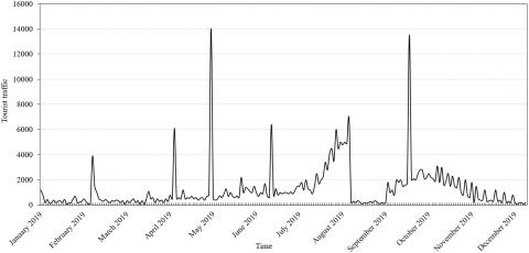
In the short term, the tourist flow in scenic areas is distributed unevenly and randomly in time and space. In the midterm and long term, however, the tourist flow distribution exhibits a certain regularity. Figure 1 presents the distribution of tourist flow in a scenic area in 2019. It can be seen that the tourist flow fluctuated obviously, due to the transitions between off-season and peak season, between weekdays and weekends, and between non-holidays and holidays. Judging by the trend of tourist flow, the off-season (April to November) differed sharply from the peak season (December to the next March) in tourist flow. In addition, the tourist flow was significantly affected by statutory holidays (e.g. New Year’s Day, Spring Festival, Labour Day, Dragon Boat Festival, National Day, and Mid-Autumn Festival), as well as the winter and summer vacations of students.
The above analysis shows that the daily tourist flow in scenic spots is featured by nonlinearity, periodicity, uneven distribution between off and peak seasons, and uneven distribution between holidays and non-holidays. To mitigate the randomness and solve the uneven distribution of short-term tourist flow in scenic areas, it is necessary to make rational classification of the factors affecting the tourist flow.
In order to eliminate the correlation between the influencing factors, this paper performs feature compression, extraction, and GRA in the following steps:
(1) Quantitative analysis of all factors
V11, V15, and V16 were set to numeric type, and measured in unit of 100 million yuan; V12, and V14 were set to numeric type, and measured in unit of yuan; V13, V211, V212, V213, and V214 were set to numeric type, and measured in unit of person-time; V221, V222, V223, V224, V231, V232, V233, V234, and V235 were one-hot encoded to digitalize the discrete categorical and hierarchical features; V24, V25, and V26 were set to numeric type, and rated according to the detailed rules on the rating of service and environmental quality; V11, and V12 were set to numeric type, and collected from the real-time weather information released by the weather station (the latter is rated against a 9-point scale from -4 to 4, where -4 means strongly uncomfortable due to extreme coldness, 0 means strongly comfortable, and 4 means strongly uncomfortable due to extreme hotness); V13, V14, and V15 were binarized, where 1 indicates that travel emergency occurs, the advertisement has been served, and the current day is a weekend/holiday, and 0 indicates the otherwise.
(2) Setting up data series
Two data series were set up: the data series of tourist flow in the scenic area reflecting tourist behaviors A={ak|k=1, 2, …, K}, and the data series of factors affecting tourist behaviors B={blk|l=1, 2, …, L; k=1, 2, …, K}.
Figure 1. The distribution of tourist flow in a scenic area in 2019
(3) Nondimensionalization
From Step (1), it can be seen that the factors in data series B differ in magnitude and dimension, owing to the difference in measuring unit. This may cause errors in the comparison process. To solve the problem, the dataset was initialized by:
${{{b}'}_{lk}}=\frac{{{b}_{lk}}}{{{b}_{l1}}}\text{ }k=1,2,...,K$ (1)
Then, the min-max normalization was introduced to standardize the deviation of the data:
${{{b}''}_{lk}}=\frac{{{{{b}'}}_{lk}}-{{{{b}'}}_{lk\text{-min}}}}{{{{{b}'}}_{lk\text{-max}}}-{{{{b}'}}_{lk\text{-min}}}}$ (2)
where, $b_{l k}^{\prime}$ is the initialized data; $b_{l k-\max }^{\prime} \text { and } b_{l k-\min }^{\prime}$ are the maximum and minimum of all data.
(4) Calculation of correlation coefficient
The maximum and minimum absolute differences between data series A and B were computed. Let α be the identification coefficient. Then, the correlation coefficient can be obtained by:
${{\delta }_{lk}}=\frac{\underset{l}{\mathop{\min }}\,\underset{k}{\mathop{\min }}\,|{{a}_{k}}-{{b}_{lk}}|+\alpha \underset{l}{\mathop{\max }}\,\underset{k}{\mathop{\max }}\,|{{a}_{k}}-{{b}_{lk}}|}{|{{a}_{k}}-{{b}_{lk}}|+\alpha \underset{i}{\mathop{\max }}\,\underset{k}{\mathop{\max }}\,|{{a}_{k}}-{{b}_{lk}}|}$ (3)
The correlation coefficient can also be expressed as the Pearson’s correlation coefficient:
${{\rho }_{lk}}=\frac{\sum\limits_{l=1}^{L}{\sum\limits_{k=1}^{K}{({{a}_{k}}-{{\mu }_{a}})}}({{b}_{lk}}-{{\mu }_{b}})}{\sqrt{\sum\limits_{k=1}^{K}{{{({{a}_{k}}-{{\mu }_{a}})}^{2}}}}\sqrt{\sum\limits_{l=1}^{L}{\sum\limits_{k=1}^{K}{{{({{b}_{lk}}-{{\mu }_{b}})}^{2}}}}}}$ (4)
(5) Calculation of relevancewhere, μa and μb are the means of data series A and B, respectively.
The relevance ri of data series B is the arithmetic mean of the correlation coefficients in the series:
${{r}_{l}}=\frac{1}{K}\sum\limits_{k=1}^{K}{\frac{{{\delta }_{lk}}+{{\rho }_{lk}}}{2}}$ (5)
The relevance ri is a number greater than 0 and smaller than 1. The closer its value is to 0, the weaker the relevance between data series A and B; the closer its value is to 1, the stronger the relevance between the two. The relevance of each factor in data series B relative to tourist flow in scenic areas can be derived from the results of formula (5) (Table 1).
Table 1. The relevance of each factor and tourist flow
|
Factor |
Relevance |
Factor |
Relevance |
Factor |
Relevance |
|
V11 |
0.6689 |
V212 |
0.7542 |
V234 |
0.6745 |
|
V12 |
0.6446 |
V213 |
0.7145 |
V235 |
0.7015 |
|
V13 |
0.6813 |
V214 |
0.6563 |
V24 |
0.6944 |
|
V14 |
0.6246 |
V221 |
0.6456 |
V25 |
0.6547 |
|
V15 |
0.6941 |
V222 |
0.6834 |
V31 |
0.6745 |
|
V16 |
0.6752 |
V223 |
0.6845 |
V32 |
0.7145 |
|
V24 |
0.6146 |
V224 |
0.6954 |
V33 |
0.6541 |
|
V25 |
0.6436 |
V231 |
0.7154 |
V34 |
|
|
V26 |
0.7262 |
V232 |
0.6852 |
V35 |
|
|
V211 |
0.6468 |
V233 |
0.7891 |
|
|
3.1 LSTM NN
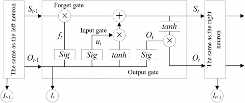
LSTM NN adds three gating units to each neuron, namely, input gate, forget gate, and output gate. Figure 2 shows the internal structure of LSTM neurons. The forget gate enables LSTM NN to selectively memorize and store important information, overcoming the long-term dependence of traditional NN. Hence, LSTM NN is suitable for processing data series B mentioned in the above section.
Figure 2. The internal structure of a LSTM neuron
The forget gate determines with a certain probability which information to discard from the neuron state. Let Ot-1 be the output of the previous neuron, and It be the input of the current neuron in LSTM NN. Then, the forget gate will read Ot-1 and It, and output a number between 0 and 1. The output number will be assigned to the state of the previous neuron St-1, indicating the probability of discarding the neuron state. If the number is 1, the neuron state will be retained fully; if the number is 0, the neuron state will be completely discarded.
${{f}_{t}}=Sigmoid({{W}_{f}}\cdot [{{O}_{t-1}},{{I}_{t}}]+{{\varepsilon }_{f}})$ (6)
Unlike the forget gate, the sigmoid activation function of the input gate determines which information needs to be updated and added to the neuron. A state vector St is generated by the tanh function to replace the state of the previous neuron St-1:
$S_{t}=f_{t} \cdot S_{t-1}+u_{t} \cdot S_{t}$ (7)
${{u}_{t}}=Sigmoid({{W}_{i}}\cdot [{{O}_{t-1}},{{I}_{t}}]+{{\varepsilon }_{i}})$ (8)
$S_{t}=\tanh \left(W_{C} \cdot\left[O_{t-1}, I_{t}\right]+\varepsilon_{C}\right)$ (9)
The output gate determines which information needs to be filtered and which needs to be output. The neuron state is processed by the tanh function. The output number, which falls between -1 and 1, is multiplied with the output of the sigmoid activation function. The final output can be expressed as formula (11):
${{h}_{t}}=Sigmoid({{W}_{h}}[{{O}_{t-1}},{{I}_{t}}]+{{\varepsilon }_{h}})$ (10)
${{O}_{t}}={{h}_{t}}\cdot \tanh ({{S}_{t}})$ (11)
Through the above analysis, this paper builds a 4-layer LSTM NN, including an input layer, an LSTM layer, a fully-connected layer, and an output layer. Among them, the input layer has three dimensions: the number of samples, the time step, and features. The LSTM layer contains n neurons with three gated units (forget gate, input gate, and output gate). Both the LSTM layer and the fully-connected layer use random orthogonal matrices for weight initialization. The difference is that the fully-connected layer adopts a linear activation function to synthesize the features extracted from the LSTM layer. The data series B obtained through GRA were taken as new features, and input to the LSTM NN for training and prediction.
The constructed model was trained in three steps: acquire valuable information through forward propagation and compute the prediction result based on reasonably set parameters; calculate the loss value; constantly correct the learning parameters through backpropagation of the loss. The loss function can be described as:
$E=\frac{1}{2}\sum\limits_{k=1}^{K}{{{({{y}_{lk}}-{{{{b}''}}_{lk}})}^{2}}}$ (12)
where, ylk is the output of the LSTM NN. To improve the distribution width of activation values in each layer, enhance the expressiveness of the network, and overcome vanishing gradients, batch normalization was added to each layer during the training, using the batches in the learning process, that is, the mean and variance of data series B, which were input in p-dimensional batches, were respectively calculated by:
$\frac{1}{p}\sum\limits_{k=1}^{p}{{{{{b}''}}_{lk}}}\to {{\eta }_{B}}$ (13)
$\sqrt{\frac{1}{p}\sum\limits_{k=1}^{p}{{{({{{{b}''}}_{lk}}-{{\eta }_{B}})}^{2}}}}\to {{\sigma }_{B}}$ (14)
Let γ be a small value. Then, the data series B can be normalized with mean of ηB and variance of σB:
$\frac{b_{l k}^{\prime \prime}-\eta_{B}}{\sqrt{\sigma_{B}^{2}+\gamma}} \rightarrow \hat{b_{l k}^{\prime \prime}}$ (15)
3.2 PSO
In the traditional PSO algorithm, N particles are randomly initialized. After t iterations, the i-th particle will move at the velocity of {vi1(t), vi2(t), …, viD(t)} in the D-dimensional search space. At this time, the particle position is {xi1(t), xi2(t), …, xiD(t)}. Starting with the current velocity and position, the i-th particle will search for the best-known individual solution pbest and the best-known global solution gbest. Let vid(t) be the velocity of the i-th particle at the t-th iteration in the d-th dimension subspace; r1, and r2 be any numbers from 0 to 1. Then, the velocity and position of particles in the swarm can be respectively updated by:
$\begin{align}& {{v}_{id}}(t+1)=\omega {{v}_{id}}(t)+{{c}_{1}}{{r}_{1}}\left[ {{p}_{best}}(t)-{{x}_{id}}(t) \right] \\& +{{c}_{2}}{{r}_{1}}\left[ {{g}_{best}}(t)-{{x}_{id}}(t) \right] \\\end{align}$ (16)
${{x}_{id}}(t+1)={{x}_{id}}(t)+{{v}_{id}}(t+1)$ (17)
where, c1 and c2 are acceleration factors; ω is the inertia weight; pbest is the best-know position of the i-th particle at the t-th iteration; gbest is the best-known position of the swarm at the t-th iteration.
In the traditional PSO algorithm, the particles may converge prematurely with the growing number of iterations t:
${{\sigma }_{PSO}}=\sqrt{{{\sum\limits_{i=1}^{N}{\left( \frac{{{\lambda }_{i}}-\bar{\lambda }}{\lambda } \right)}}^{2}}}\le \beta $ (18)
where, β is a preset threshold; σPSO is the variance of swarm fitness. To limit the variance, a normalization factor called fitness λ is introduced:
$\lambda=\left\{\begin{array}{l}
\max \left|\lambda_{i}-\bar{\lambda}\right|, \max \left|\lambda_{i}-\bar{\lambda}\right|>1 \\
1, \max \left|\lambda_{i}-\bar{\lambda}\right|<1
\end{array}\right.$ (19)
The particles need to be disturbed more intensely to prevent premature convergence. The exploration and search abilities of particles can be controlled by adjusting the inertia weight ω, such that the particles could get out of the local optimum trap. Let tmax be the maximum number of iterations for the swarm. Then, ω can be expressed as:
$\omega ={{\omega }_{\max }}-\frac{t\cdot ({{\omega }_{\max }}-{{\omega }_{\min }})}{{{t}_{\max }}}$ (20)
where, ωmin and ωmax are the minimum and maximum of inertia weight, respectively. Traditionally, ω is adjusted nonlinearly with the Gaussian function:
$\omega ={{\omega }_{\min }}+({{\omega }_{\max }}-{{\omega }_{\min }}\times \exp \left[ \frac{-{{t}^{2}}}{0.2\times {{t}_{\max }}{{)}^{2}}} \right]$ (21)
However, this gradual adjustment approach will weaken the optimization performance of the swarm. In the early iterations, the particles have relatively weak local search ability, and converge rather slowly. It is difficult for a particle to make detailed searches in the global best-known area. In the later iterations, the particles have relatively weak global search ability, failing to jump out of the local optimum trap. To solve the problems, the adjustment method for ω was optimized as follows, considering the difference between the variances of swarm fitness in adjacent iterations:
$\omega =\left\{ \begin{align} & {{\omega }_{\max }}-({{\omega }_{\max }}-{{\omega }_{\min }})\times \frac{\ln \left[ \bar{\lambda }(t+1) \right]-\ln \left[ {{\lambda }_{i}}(t+1) \right]}{\ln \left[ \bar{\lambda }(t+1) \right]},\Delta {{\sigma }_{PSO}}>{{\lambda }_{i}}(t+1)\ge \bar{\lambda } \\ & {{\omega }_{\min }},{{\lambda }_{i}}(t+1)<\min (\begin{matrix} {\bar{\lambda }} & \Delta {{\sigma }_{PSO}} \\\end{matrix}) \\ & {{\omega }_{\max }},{{\lambda }_{i}}(t+1)>\max (\begin{matrix} {\bar{\lambda }} & \Delta {{\sigma }_{PSO}} \\\end{matrix}) \\ & {{\omega }_{\min }}-({{\omega }_{\max }}-{{\omega }_{\min }})\times \frac{\ln \left[ {{\lambda }_{i}}(t+1) \right]-n\left[ \bar{\lambda }(t+1) \right]}{\ln \left[ {{\lambda }_{i}}(t+1) \right]},\Delta {{\sigma }_{PSO}}<{{\lambda }_{i}}(t+1)<\bar{\lambda } \\\end{align} \right.$ (22)
where, λi(t+1) is the fitness of the i-th particle at the t+1-th iteration; λ is the mean fitness of the swarm at the t-th iteration. It can be seen that, if ΔσPSO is relatively large, the particle distribution is dispersed, and ω needs to be reduced to accelerate the convergence; if λi is greater than`λ, the particle is outside the best-known area, and ω needs to be increased to relocate the optimal solution; if λi is smaller than λ, the particle has good learning ability, and ω needs to be further reduced to find the optimal solution quickly; if ΔσPSO is extremely small, the particle swarm will converge prematurely, and the particles need to be disturbed, making the swarm more diverse.
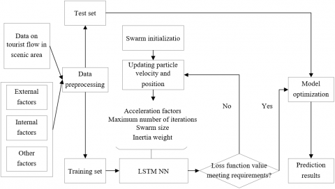
Figure 3 illustrates the structure of the LSTM NN optimized by the adaptive PSO algorithm, in which the inertia weight is based on log function. Firstly, the LSTM NN parameters are adjusted by the adaptive PSO algorithm, that is, the global best-known position is transferred to the Ot-1 and It of the LSTM for calculation. Then, the loss function of LSTM is taken as the fitness of the adaptive PSO algorithm, and used to update the velocity and position of each particle in the swarm. The specific workflow of the proposed model is as follows:
(1) Initialize the parameters of the adaptive PSO algorithm: swarm size, maximum number of iterations, acceleration factors, minimum inertia weight, maximum inertia weight, initial velocity, and initial position.
(2) Define the parameters of LSTM NN, and transfer the initial position of each particle to the Ot-1 and It of the LSTM. Take the loss function value on the test set as the initial fitness λ0 of the particle, calculate the value of $\bar{\lambda}$, and search for the best-known individual and global solutions pbest and gbest.
(3) Calculate the inertia weight by formula (22), and update the velocity and position of each particle by formulas (16) and (15), respectively. Judge whether the updated velocity and position surpass the limit: If xid(t+1)>xmax, vid(t+1)>vmax, then xid(t+1)=xmax, vid(t+1)=vmax; if xid(t+1)<xmin, vid(t+1)<vmin, then xid(t+1)=xmin, vid(t+1)=vmin.
(4) Recalculate λi(t+1), and update pbest and gbest. If λi(t+1) is better than pbest, replace pbest with λi(t+1); If λi(t+1) is better than gbest, replace gbest with λi(t+1).
(5) Judge if the termination condition is satisfied. If not, return to Step 3 and repeat Steps 3-5 until the condition is satisfied; if yes, terminate the iteration, and output the global optimal solution.
(6) Import the global optimal solution to the LSTM NN, kicking off a new round of training and prediction.
Figure 3. The structure of the proposed model
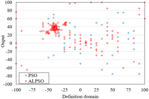
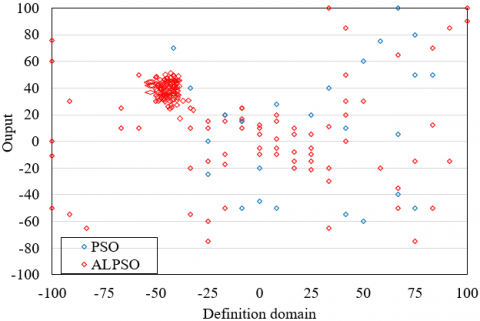
(a) 30 iterations
(b) 150 iterations
Figure 4. The particle distribution in the search process
The particle distributions of the traditional PSO algorithm and the proposed adaptive PSO algorithm were recorded, aiming to demonstrate the ability of our algorithm to optimize NN. The particle distributions after 30 and 150 iterations are presented in Figures 4(a) and 4(b), respectively. Compared with the traditional PSO algorithm, the proposed algorithm expands the search range of particles in the early and later iterations, during the search for the optimal solution. In this way, our algorithm effectively prevents particles from falling into local optimum trap and avoids premature convergence. Moreover, the particles of our algorithm clustered around the optimal solution in the early phase of the search, indicating that our algorithm ensures fast and effective convergence.
To verify the performance of the proposed LSTM NN, this paper carries out simulations on Matlab2010, with the dataset of daily tourist flow in a scenic area from 2018 to 2019 as the training set, and the dataset of daily tourist flow in that scenic area from January to September 2020 as the test set. The original data series exist as a 3×1,578 matrix.
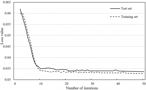
The convergence of loss function in the LSTM NN is displayed in Figure 5. Obviously, the loss values on test set and training set both tended to be stable at around 30 iterations, indicating that the network has basically converged. Thus, the maximum number of iterations was set to 40. The loss values on test set and training set were about 0.0342 and 0.0328, respectively.
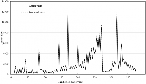
Figure 6 provides the prediction results of our NN on the tourist flow in the scenic area. It can be seen that the predicted values basically overlapped with the actual values. The prediction accuracy was still desirable, even if the tourist flow surged up on holidays in May and October.
Furthermore, our model was compared with several time series prediction methods, including RF, SVM, recurrent neural network (RNN), the LSTM optimized by traditional PSO (PSO-LSTM). The prediction results and errors of these methods are given in Tables 2 and 3, respectively. As shown in Table 2, the peak season of the scenic area lasts from April to October, according to the prediction results of all contrastive methods. Hence, the predictions are basically consistent with the actual situation.
Figure 5. The convergence of loss function in the LSTM NN
Figure 6. The prediction results of our model
Table 2. The comparison of prediction results
|
Month |
RF |
SVM |
RNN |
PSO-LSTM |
Our model |
|
January |
2,765 |
2,846 |
2,798 |
2,754 |
2,854 |
|
February |
2,697 |
2,721 |
2,654 |
2,665 |
2,754 |
|
March |
2,865 |
2,789 |
2,795 |
2,855 |
2,841 |
|
April |
3,965 |
3,843 |
3,836 |
3,912 |
3,979 |
|
May |
6,589 |
7,635 |
8,754 |
7,513 |
9,549 |
|
June |
4,258 |
4,167 |
4,379 |
5,290 |
4,947 |
|
July |
5,659 |
5,477 |
5,275 |
5,145 |
5,096 |
|
August |
5,258 |
5,159 |
5,359 |
5,058 |
5,357 |
|
September |
6,059 |
5,541 |
6,214 |
6,145 |
6,248 |
|
October |
10,978 |
10,845 |
11,012 |
10,956 |
10,988 |
|
November |
4,245 |
4,169 |
4,354 |
5,214 |
4,558 |
|
December |
3,895 |
3,954 |
3,125 |
3,732 |
3,854 |
Table 3. The prediction errors of different models
|
Method |
RMSE |
MAE |
MAPE |
R2 |
|
RF |
1,645.89 |
1,187.36 |
98.65 |
-2.65 |
|
SVM |
502.62 |
293.15 |
56.89 |
0.98 |
|
RNN |
384.26 |
157.38 |
16.58 |
0.94 |
|
PSO-LSTM |
321.85 |
208.65 |
26.54 |
0.96 |
|
Our method |
193.21 |
96.46 |
6.98 |
0.93 |
Note: RMSE, MAE, MAPE, and R2 are short for root mean square error, mean absolute error, mean absolute percentage error, and coefficient of determination, respectively.
As shown in Table 3, the RF, which is based on random sampling, had the greatest prediction error. This means RF is not a good choice for the prediction of tourist flow with strong nonlinear features. The PSO-LSTM had lower errors than SVM and RNN, indicating that LSTM NN can effectively overcome the long-term dependence in time series data. Our model boasted the smallest errors, because the redundant information is removed through GRA of influencing factors. This dimensionality reduction treatment ensures the extraction of important information from the data series, while improving the training effect of the NN. The ultralow MAPE (<6.98) fully demonstrates the effectiveness of our model.
This paper fully explores and further optimizes the existing AI methods, and comes up with a tourist flow prediction model for scenic areas based on the PSO of NN. Firstly, the authors built up a system of factors affecting the tourist flow in scenic areas, and eliminated the factors with low relevance through GCA. On this basis, the LSTM NN was optimized with adaptive PSO, creating a tourist flow prediction model for scenic areas. The workflow of the proposed model was detailed. Experimental results show that the proposed adaptive PSO algorithm can effectively prevent particles from falling into local optimum trap and avoids premature convergence. Furthermore, our model was compared with time series prediction methods like RF, SVM, RNN, and PSO-LSTM. The comparison shows that our model can greatly enhance the prediction accuracy of tourist flow in scenic areas, and achieve desirable effect in peak season and on holidays.
[1] Kang, S., Lee, G., Kim, J., Park, D. (2018). Identifying the spatial structure of the tourist attraction system in South Korea using GIS and network analysis: An application of anchor-point theory. Journal of Destination Marketing & Management, 9: 358-370. https://doi.org/10.1016/j.jdmm.2018.04.001
[2] Expósito, A., Mancini, S., Brito, J., Moreno, J.A. (2019). A fuzzy GRASP for the tourist trip design with clustered POIs. Expert Systems with Applications, 127: 210-227. https://doi.org/10.1016/j.eswa.2019.03.004
[3] Tripathy, A.K., Tripathy, P.K., Ray, N.K., Mohanty, S.P. (2018). iTour: The future of smart tourism: An IoT framework for the independent mobility of tourists in smart cities. IEEE Consumer Electronics Magazine, 7(3): 32-37. https://doi.org/10.1109/MCE.2018.2797758
[4] Tang, Z., Liu, L., Li, X.H., Shi, C.B., Zhang, N., Zhu, Z.J., Bi, J. (2019). Evaluation on the eco-innovation level of the tourism industry in Heilongjiang Province, China: From the perspective of dynamic evolution and spatial difference. International Journal of Sustainable Development and Planning, 14(3): 202-215. https://doi.org/10.2495/SDP-V14-N3-202-215
[5] Nunes, N., Ribeiro, M., Prandi, C., Nisi, V. (2017). Beanstalk: a community based passive wi-fi tracking system for analysing tourism dynamics. EICS '17: Proceedings of the ACM SIGCHI Symposium on Engineering Interactive Computing Systems, pp. 93-98 https://doi.org/10.1145/3102113.3102142
[6] Gálvez, J.C.P., Granda, M.J., López-Guzmán, T., Coronel, J.R. (2017). Local gastronomy, culture and tourism sustainable cities: The behavior of the American tourist. Sustainable Cities and Society, 32: 604-612. https://doi.org/10.1016/j.scs.2017.04.021
[7] Navío-Marco, J., Ruiz-Gómez, L.M., Sevilla-Sevilla, C. (2018). Progress in information technology and tourism management: 30 years on and 20 years after the internet-Revisiting Buhalis & Law's landmark study about eTourism. Tourism Management, 69: 460-470. https://doi.org/10.1016/j.tourman.2018.06.002
[8] Bu, N., Kong, H., Ye, S. (2020). County tourism development in China: A case study. Journal of China Tourism Research, 1-24. https://doi.org/10.1080/19388160.2020.1761501
[9] Dale, N.F. (2019). Gender and other factors that influence tourism preferences. Gender Economics: Breakthroughs in Research and Practice, 454-471.
[10] Lee, H., Lee, J., Chung, N., Koo, C. (2018). Tourists’ happiness: Are there smart tourism technology effects? Asia Pacific Journal of Tourism Research, 23(5): 486-501. https://doi.org/10.1080/10941665.2018.1468344
[11] Divisekera, S., Nguyen, V.K. (2018). Determinants of innovation in tourism evidence from Australia. Tourism Management, 67: 157-167. https://doi.org/10.1016/j.tourman.2018.01.010
[12] Leung, R., Vu, H.Q., Rong, J., Miao, Y. (2016). Tourists visit and photo sharing behavior analysis: A case study of Hong Kong temples. Information and Communication Technologies in Tourism 2016, 197-209. https://doi.org/10.1007/978-3-319-28231-2_15
[13] Vu, H.Q., Leung, R., Rong, J., Miao, Y. (2016). Exploring park visitors’ activities in Hong Kong using geotagged photos. Information and Communication Technologies in Tourism 2016, 183-196. https://doi.org/10.1007/978-3-319-28231-2_14
[14] Lim, K.H., Chan, J., Karunasekera, S., Leckie, C. (2019). Tour recommendation and trip planning using location-based social media: A survey. Knowledge and Information Systems, 60: 1247-1275. https://doi.org/10.1007/s10115-018-1297-4
[15] Cenamor, I., de la Rosa, T., Núñez, S., Borrajo, D. (2017). Planning for tourism routes using social networks. Expert Systems with Applications, 69: 1-9. https://doi.org/10.1016/j.eswa.2016.10.030
[16] Kotiloglu, S., Lappas, T., Pelechrinis, K., Repoussis, P.P. (2017). Personalized multi-period tour recommendations. Tourism Management, 62: 76-88. https://doi.org/10.1016/j.tourman.2017.03.005
[17] Mir, T. (2017). Role of social media in tourism: a literature review. International Journal for Research in Applied Science and Engineering Technology, 5(11), 633-635. https://doi.org/10.22214/ijraset.2017.11099
[18] Kim, J., Thapa, B., Jang, S. (2019). GPS-based mobile exercise application: An alternative tool to assess spatio-temporal patterns of visitors' activities in a national park. Journal of Park & Recreation Administration, 37(1): 124-134. https://doi.org/10.18666/JPRA-2019-9175
[19] Park, J.H., Lee, C., Yoo, C., Nam, Y. (2016). An analysis of the utilization of Facebook by local Korean governments for tourism development and the network of smart tourism ecosystem. International Journal of Information Management, 36(6): 1320-1327. https://doi.org/10.1016/j.ijinfomgt.2016.05.027
[20] Huertas, A., Moreno, A., My, T.H. (2019). Which destination is smarter? Application of the (SA) 6 framework to establish a ranking of smart tourist destinations. International Journal of Information Systems and Tourism (IJIST), 4(1): 19-28.
[21] Chung, N., Lee, H., Kim, J.Y., Koo, C. (2018). The role of augmented reality for experience-influenced environments: The case of cultural heritage tourism in Korea. Journal of Travel Research, 57(5): 627-643. https://doi.org/10.1177/0047287517708255
[22] tom Dieck, M.C., Jung, T. (2018). A theoretical model of mobile augmented reality acceptance in urban heritage tourism. Current Issues in Tourism, 21(2): 154-174. https://doi.org/10.1080/13683500.2015.1070801
[23] Del Vecchio, P., Mele, G., Ndou, V., Secundo, G. (2018). Creating value from social big data: Implications for smart tourism destinations. Information Processing & Management, 54(5): 847-860. https://doi.org/10.1016/j.ipm.2017.10.006
[24] Wise, N., Heidari, H. (2019). Developing smart tourism destinations with the internet of things. Big Data and Innovation in Tourism, Travel, and Hospitality, 21-29. https://doi.org/10.1007/978-981-13-6339-9_2