Hao Lin | Leixiao Li* | Hui Wang | Yongsheng Wang | Zhiqiang Ma
© 2020 IIETA. This article is published by IIETA and is licensed under the CC BY 4.0 license (http://creativecommons.org/licenses/by/4.0/).
OPEN ACCESS
Traffic flow prediction is popular research of ITS. Traffic flow prediction models based on machine learning have recently been widely applied. In this study, we use machine learning algorithms, heuristic algorithms, and parallelization technology to propose a traffic flow prediction model based on Relevance Vector Machine called Genetic Algorithm and Particle Swarm Optimization based on spark parallelization optimized Combined kernel RVM (SPGAPSO-CKRVM). First, combined kernel functions are constructed based on common kernel functions. Second, a parameter optimization algorithm is proposed to optimize the parameters of combined kernel functions by Genetic Algorithm and Particle Swarm Optimization. To reduce time consumed by the parameter optimization algorithm, we parallel the parameter optimization algorithm by Spark. Finally, the proposed model is verified with the real data of Whitemud Drive in Canada. The experimental results indicate that SPGAPSO-CKRVM has greater accuracy than other prediction models and parallelization technology reduce time consumed by the parameter optimization algorithm significantly.
traffic flow prediction, relevance vector machine, combined kernel function, parameter optimization, Spark
The predecessor of Intelligent Traffic Systems (ITS) is Intelligent Vehicle Highway System (IVHS). ITS combines with advanced science and technology such as information technology, sensor technology, automatic control theory, operational research, and artificial intelligence to improve transportation industry. Applications and research of ITS involve highway, railway, civil aviation, water carriage and other modes of transportation [1-3]. Traffic flow prediction is a part of ITS. Travelers and government sectors can receive real-time traffic information and basis of decision for traffic congestion by accurate and reliable results of traffic flow prediction. Sensor systems installed on various road types provide traffic network flow, speed, lane occupancy and other information to realize short-term traffic flow prediction. How to improve the accuracy of traffic flow prediction has always been a research focus in ITS [4, 5]. Traffic flow prediction is a typical time series prediction problem [6]. Machine learning and deep learning provide significant solution for solving complicated time series prediction problems. At present, many machine learning and deep learning algorithms have been used to predict traffic flow, but the accuracy and efficiency of algorithms still have room for improvement. Relevance vector machine (RVM) has extremely short testing speed and excellent generalization ability [7]. RVM is widely used in traffic flow prediction due to periodicity, tidal nature and nonlinearity of traffic flow and demand for real-time prediction [4]. Based on the above reasons, this paper combines RVM, heuristic algorithms and parallelization technology to construct an accurate and efficient traffic flow prediction model called SPGAPSO-CKRVM. The main contributions of this paper are summarized as follows:
• First, we implement RVM based on common kernel functions and combined kernel functions. A new measurement called Peak Hours Accuracy is proposed to evaluate capability of kernel function in traffic flow prediction. According to the experimental results, we select a combined kernel function which combine Polynomial kernel and Gaussian kernel as the kernel function of RVM to realize prediction model.
• Second, for the parameter optimization of combined kernel functions, Genetic Algorithm (GA) and Particle Swarm Optimization (PSO) are used to build a hybrid parameter optimization algorithm in this paper. Because the parameter optimization algorithm is time-consuming, we use parallelization technology based on Spark to parallel parameter optimization algorithm to improve efficiency of algorithm. We name this traffic flow prediction model SPGAPSO-CKRVM. This is the first time to introduce Spark into parameter optimization of RVM.
• Third, we proved that SPGAPSO-CKRVM has better prediction accuracy and efficiency than traditional methods by analyzing experimental results.
The remainder of this paper is organized as follows: the related works are discussed in Section 2. Section 3 outlines the principle of RVM. Section 4 introduces traffic flow prediction model called SPGAPSO-CKRVM. Section 5 carries out experiments and analyzes the experimental results. Finally, Section 6 draws the conclusion.
There are two main types of research about traffic flow prediction. One type is driven by models. They predict traffic flow by using Auto Regression Moving Average Model (ARMA) [8], Autoregressive Integrated Moving Average Model (ARIMA) [9], Kalman Filtering [10] and other models. These methods usually assume that time series data is generated by a linear process. So, they establish the relationship among time series data based on a linear relation. Therefore, although the calculation is simple, the accuracy is poor.
The second one such as Support Vector Machine (SVM), Recurrent Neural Network (RNN), RVM and other machine learning and deep learning algorithms is driven by data. Cao and Xu [11] proposed a traffic flow prediction method based on SVM optimized by PSO. It is proved that SVM combined with intelligent algorithms is suitable for prediction traffic flow. Tian et al. [12] proposed a novel approach based on Long Short-Term Memory (LSTM) to predict traffic flow. In addition, the multiscale temporal smoothing is employed to infer lost data in this approach. Fu et al. [13] used LSTM and Gated Recurrent Unit (GRU) to forecast traffic flow respectively. The experimental results show that GRU outperforms LSTM and is significantly better than ARIMA. In recent years, deep models based on deep learning gradually favored by scholars. The deep models improve capability by a new method which extracts the feature of traffic flow information before prediction traffic flow. CNN-LSTM is the most popular one among the deep models [14]. CNN-LSTM extracts the feature such as spatiotemporal feature and periodic feature by convolutional layer to generate a new feature data set. Then input it into LSTM for prediction traffic flow [15]. Liu et al. [16] proposed CNN-Bi-LSTM by replacing LSTM in CNN-LSTM with Bidirectional Long Short Memory Network(Bi-LSTM). CNN-LSTM has better accuracy than other deep learning algorithms based on RNN. Extracting feature by convolutional layer can be regarded as reducing dimensionality of data. So, CNN-LSTM has better efficiency than LSTM and GRU, but the advantage is not significant in traffic flow prediction.
RVM was proposed as a sparse probability model based on Bayesian frame in 2000. RVM has extremely short testing speed and prediction accuracy similar to SVM, LSTM and GRU. Therefore, RVM is often regarded as an optimized version of SVM. The parameter optimization of RVM kernel functions is an unavoidable problem for every research about RVM. Accuracy of RVM without parameter optimization is not ideal. For this problem, Jin and Hui [17] used GA to optimize RVM to prove that the intelligent algorithms improve capability of RVM. Shen et al. [18] proposed a hybrid algorithm called Chaos Simulated Annealing Algorithm (CSA) and used it to optimize RVM to predict traffic flow. This method has better prediction accuracy than model-driven methods such as seasonal auto regressive integrated moving average (SARIMA). Shen et al. [19] also used CSA to optimize RVM. By comparing with RVR-GA, SVR-GA, BPNN-GA and other algorithms, Shen et al. proved that their method has better capability. They only used the advantage that RVM has short testing time in their respective prediction models without considering the efficiency of parameter optimization algorithms of RVM. In previous research, for machine learning algorithms such as SVM and RVM, we found that the time consumed by the parameter optimization algorithm accounts for 80%-95% of the overall training time [4]. The efficiency of parameter optimization algorithms greatly affects the efficiency of overall algorithm.
Currently, the efficiency of parameter optimization algorithms in machine learning is researched less. Most of this research focus on Grid Search (GS). Wu and Ning [20] used Hadoop to parallel GS and used it to optimize SVM. This method can only increase the efficiency of GS by 50%. Li et al. [21] paralleled GS by Spark, based on this design, proved that using of Spark parallelization technology can improve the efficiency of parameter optimization algorithms significantly without reducing its accuracy.
RVM is a supervised learning algorithm proposed by Micnacl E. Tipping in 2000. RVM has the advantages of SVM and overcomes the disadvantages of SVM such as support vectors too many to calculate slowly, long testing time, kernel functions must meet Mercer’s theorem [7]. Micnacl E. Tipping realize RVM as a sparse model with Automatic Relevance Determination (ARD) to reflect the central features of data and reduce calculation in testing step. The basic mathematical model of RVM can be represented as:
$y(x, \omega)=\sum_{i=1}^{N} \omega_{i} K\left(X, X_{i}\right)+\varepsilon_{n}$ (1)
where, ωi is weight of sample. ωi is non-zero when Xi belongs to the relevance vector. K(X, Xi) is kernel function of RVM. N is total number of samples. εn is Gaussian noise that follows Gaussian distribution (0, σ2). For tn=y(x, ω)+εn, since tn is independently distributed, the likelihood function of training set as follows:
$\begin{array}{c}
P\left(t \mid \omega, \sigma^{2}\right) \sim N\left(0, \sigma^{2}\right) \\
P\left(t \mid \omega, \sigma^{2}\right)=\left(2 \pi \sigma^{2}\right)^{-\frac{N}{2}} \exp \left(-\frac{1}{2 \sigma^{2}}\|t-\phi \omega\|^{2}\right)
\end{array}$ (2)
If Eq. (2) is directly maximized by Structural Risk Minimization (SRM) will cause serious overfitting problems. Therefore, $\omega_{i}$ should be defined to satisfy the Gaussian prior probability distribution. It is as follows:
$\begin{array}{c}
P(\omega \mid \alpha)=\prod_{i=0}^{N} N\left(\omega_{i} \mid 0, \alpha_{i}^{-1}\right) \\
=\prod_{i=0}^{N} \sqrt{\frac{\alpha_{i}}{2 \pi}} \exp \left(-\frac{\alpha_{i}}{2} \omega_{i}^{2}\right)
\end{array}$ (3)
where, α=[α0, α1, α2, …, αN]T is hyperparameter that determines the prior distribution of ωi. The posterior distribution of ωi can be calculated by Bayesian formula as follows:
$P\left(\omega \mid t, \alpha, \sigma^{2}\right)=\frac{P\left(t \mid \omega, \sigma^{2}\right) P(\omega \mid \alpha)}{P\left(t \mid \alpha, \sigma^{2}\right)}$ (4)
where, P(ω|t, α, σ2) follows Gaussian distribution. It’s mean value and covariance can be represented as:
$\mu=\sigma^{-2} \rho \phi^{T} t$ (5)
$\rho=\left(\sigma^{-2} \phi^{T} \phi+A\right)^{-1}, A=\operatorname{diag}\left(\alpha_{0}, \alpha_{1}, \ldots, \alpha_{N}\right)$ (6)
For estimating weights of the model, the optimal value of hyperparameters should be estimated firstly. Suppose $\alpha$ follows the Gamma Distribution, the likelihood distribution of hyperparameters can be represented as:
$P\left(t \mid \alpha, \sigma^{2}\right)=\int P\left(t \mid \omega, \sigma^{2}\right) P(\omega \mid \alpha) d \omega$ (7)
We can calculate an approximate solution $\left(\alpha_{M}, \sigma_{M}^{2}\right)$ by maximizing P(t|α, σ2). Then, repeat Eq. 8 by MacKay [22] and update µ and ρ simultaneously until meet the convergence condition.
$\alpha_{i}^{\text {new}}=\frac{\gamma_{i}}{\mu_{i}^{2}},\left(\sigma^{2}\right)^{\text {new}}=\frac{\|t-\rho \mu\|^{2}}{N-\rho_{i} \gamma_{i}}$ (8)
Most of αi tend to infinity and ωi corresponding to αi tend to zero during the iteration. That is why RVM is a sparse probability model. Where, samples learned by non-zero ωi called relevance vector. After the convergence process, we can estimate xp by Eq. (9) and Eq. (10).
$P\left(t_{p} \mid t, \alpha_{M}, \sigma_{M}^{2}\right)=N\left(t_{p} \mid y_{p}, \sigma_{p}^{2}\right)$ (9)
$y_{p}=\mu^{T} \phi\left(x_{p}\right), \sigma_{p}^{2}=\sigma_{M}^{2}+\phi\left(x_{p}\right)^{T} \rho \phi\left(x_{p}\right)$ (10)
where, xp is the data to be tested. yp is predictive value of RVM.
RVM has same functional form as SVM and deal with nonlinear problems by Kernel Trick. But RVM has shorter testing time than SVM because it is a sparse probability model and the accuracy is similar to SVM. So RVM is more suitable for predicting traffic flow.
4.1 Combined kernel
In the current study, most of RVM used single kernel functions such as Linear kernel, Polynomial kernel, Gaussian kernel, Sigmoid kernel, and Laplace kernel to complete the mapping process in feature space. Where, Linear kernel and Polynomial kernel have better capability in single-dimensional and low-dimensional problems. Gaussian kernel and Sigmoid kernel are used widely in high-dimensional problems and classification problems. Single kernel functions have poor capability when the samples are large and distributed unevenly in the high-dimensional space [23, 24]. So, we combine single kernel functions to construct a combined kernel function. Combined kernel functions as shown in the Eq. (11) and Eq. (12).
$\begin{aligned}
f\left(x, x_{i}\right) &=\exp \left(-\frac{\left\|x-x_{i}\right\|^{2}}{2 \sigma^{2}}\right) \lambda \\
&+(1-\lambda)\left[\gamma\left(x x_{i}+1\right)^{d}+c\right]
\end{aligned}$ (11)
$\begin{aligned}
f\left(x, x_{i}\right) &=\exp \left(-\frac{\left\|x-x_{i}\right\|}{2 \sigma^{2}}\right) \lambda \\
&+(1-\lambda)\left[\gamma\left(x x_{i}+1\right)^{d}+c\right]
\end{aligned}$ (12)
There is no need to prove availability of the combined kernel functions shown in Eq. (11) and Eq. (12), because kernel functions of RVM do not need to meet Mercer’s theorem. The combined kernel functions make RVM get local learning ability of Gaussian kernel and Laplace kernel and generalization of Polynomial kernel. Where, σ is width of kernel function. γ determines the distribution of the data in high-dimensional space. λ is weight coefficient. It meets 0≤λ≤1.
4.2 Input of model
In the current study, the time span of short-term traffic flow prediction is not shorter than 10 min. The shorter the time span, the more valuable the model. So, we deal with traffic flow data into 5 min time span. The input of the prediction model designed in this paper is:
$X=\left[\begin{array}{l}\overrightarrow{x_{1}} \\ \overrightarrow{x_{2}} \\ \cdots \\ \overrightarrow{x_{N}}\end{array}\right]=$$\left[\begin{array}{cccccccc}x_{1}^{i-7 n, j} & x_{1}^{i-7 n+7, j} &\ldots & x_{1}^{i-7, j} & x_{1}^{i, j-m} &\ldots & x_{1}^{i, j-1} & x_{1}^{i, j} \\ x_{2}^{i-7 n, j} & x_{2}^{i-7 n+7, j} & \ldots & x_{2}^{i-7, j} & x_{2}^{i, j-m} & \ldots & x_{2}^{i, j-1} & x_{2}^{i, j} \\ \cdots & \ldots & \ldots & \ldots & \ldots & \ldots & \ldots & \ldots \\ x_{N}^{i-7 n, j} & x_{N}^{i-7 n+7, j} & \ldots & x_{N}^{i-7, j} & x_{N}^{i, j-m} & \ldots & x_{N}^{i, j-1} & x_{N}^{i, j}\end{array}\right]$ (13)
where, $\left(x_{1}^{i, j}, x_{2}^{i, j}, \ldots, x_{N}^{i, j}\right)^{T}$ is the prediction target. i represents the date. j represents the time points. (xi,j-m, xi,j-m-1, …, xi,j-1) represents the traffic volume at m time points before the jth time point in the ith day. (xi-7n,j, xi-7n+7,j, …, xi-7,j) represents the traffic volume at the jth time point in n days before the ith day. The reason for this is, the traffic volume at a certain time is often affected by the traffic volume at the same time in the previous n weeks. m is often called “training step” or “time-window”. m and n are positive integers. According to the experimental data we used, we set m=10, n=3.
4.3 Parameter optimization algorithm of RVM based on combined kernel
Parameter optimization problem of RVM based on combined kernel is different from general parameter optimization problem of RVM. λ in the combined kernel function as shown in Eq. (11) and Eq. (12) is also hyperparameter which need to be optimized. The mathematical model of the parameter optimization algorithm proposed in this paper as follows:
$P=\left\{\sigma_{\text {best}}, \lambda_{\text {best}}, \gamma_{\text {best}}\right\}$ (14)
We design the parameter optimization algorithm of RVM with GA and PSO. First, initialize two populations randomly and run GA and PSO respectively based on the two populations to generate next generation population. A population represents many P. Then, choose the better one of the two populations by calculating the individual fitness in each iteration. Use the population which is chosen as input for the next iteration. Where, the update formula of σbest as follows:
$\sigma_{\text {best}}=\left\{\begin{array}{l}
\sigma_{\text {gabest}}, \text {fitness}_{g a} \geq \text {fitness}_{\text {pso}} \\
\sigma_{\text {psobest}}, \text {fitness}_{g a} \leq \text {fitness}_{\text {pso}}
\end{array}\right.$ (15)
The update formulas of γbest and λbest are similar to Eq. (15). Because both GA and PSO optimize parameter with iteration, the parameter optimization algorithm designed by us takes advantages of GA and PSO simultaneously. Input {σbest, λbest, γbest} obtained by updating of σbest, γbest and λbest as parameters of RVM to calculate the accuracy pAccuracy of prediction model. Define pAccuracy as the objective function of the parameter optimization problem. We get:
$\max p_{\text {Accuracy}}=\operatorname{RVM}\left\{\sigma_{\text {best}}, \lambda_{\text {best}}, \gamma_{\text {best}}\right\}$
$\text { s.t. }\left\{\begin{aligned}
2^{\sigma_{\min }} & \leq \sigma_{\text {best}} \leq 2^{\sigma_{\max }} \\
\gamma_{\min } & \leq \gamma_{\text {best}} \leq \gamma_{\max } \\
0 & \leq \lambda_{\text {hest}} \leq 1
\end{aligned}\right.$ (16)
where, 2σmin and 2σmax mean variation range of σbest. Generally, 2σmin=-8 and 2σmax =8. γmin and γmax mean variation range of γbest. Generally, γmin=0 and γmax=+∞. Terminate iteration of parameter optimization algorithm until the termination condition is met. The termination condition as follows:
$\begin{array}{c}
\min \left\{\text {fitness}_{g a}, \text {fitness}_{\text {pso}}\right\} \leq \text {fitness}_{\text {min}} \\
\text {or } T \leq T_{\max }
\end{array}$ (17)
where, fitnessmin is minimum fitness (i.e. acceptable minimum error of prediction model). T is times of iteration. Tmax is maximum times of iteration.
4.3.1 Details of GA
For parameter optimization algorithm of RVM, Binary encoding is the most common coding method. GA evaluates each P by fitness function to guide parameter optimization into a good direction. We use mean-square error (MSE) of RVM as fitness function.
After calculating fitness, choose individuals in population by Roulette Wheel Selection. Then, use selected individuals to generate a new population with crossover and mutation [25].
4.3.2 Details of PSO
PSO evaluates each P by MSE of RVM similarly as GA. Find individual extremum and global extremum by the results of calculating fitness [26]. Then update the speed and position of each particles by Eq. (18) and Eq. (19).
$v=v_{i}+c_{1} r_{1}\left(p_{\text {best}}-x_{i}\right)+c_{2} r_{2}\left(G_{\text {best}}-x_{i}\right)$ (18)
$x=x_{i}-v_{i}$ (19)
where, v is updated velocity of particle. x is updated position of particle. vi is current velocity of particle. xi is current position of particle. c1 and c2 are called learning factor and determine the learning step. r1 and r2 are random numbers from zero to one. pbest is individual extremum. Gbest is global extremum.
4.4 Time-consuming analysis of parameter optimization algorithm
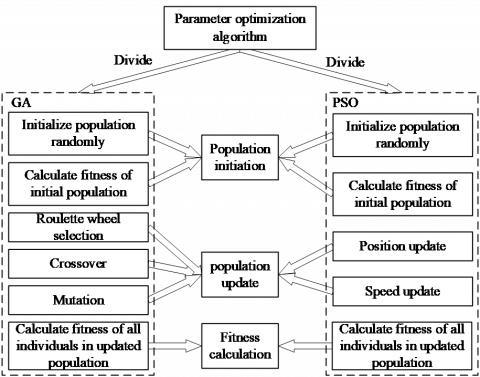
GA and PSO in parameter optimization algorithm designed in this paper can be divided into three parts—population initiation, population update and fitness calculation. The structure of parameter optimization algorithm is shown in Figure 1.
Figure 1. The structure of parameter optimization algorithm
As Figure 1 shows that population initiation includes two parts—initialize the population randomly and calculate fitness of the initial population. Population update includes five parts—roulette wheel selection, crossover, mutation, speed update and position update. Fitness calculation is responsible for calculating the fitness of all individuals in the updated population.
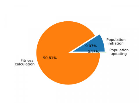
Run parameter optimization algorithm designed in this paper twenty times to collect the time consumed by each part in the algorithm. Where, Tmax=20 and population size is 10. The results are shown in Figure 2.
Figure 2. Time consumed by each part in parameter optimization algorithm
The Figure 2 shows that fitness calculation consumes the most time and accounts for more than 90% of the total time. The time spends on population update with complex calculation logic only accounts for about 0.1% of the total time. So, for fitness calculation is the most time-consuming, we parallel parameter optimization algorithm to reduce runtime of calculation fitness by Spark.
4.5 Parallel design
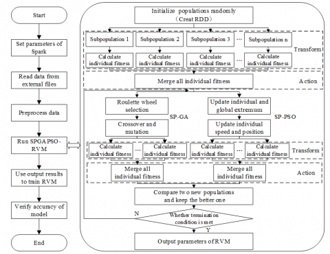
Spark is a fast and universal computing engine designed for processing largescale data [27]. Spark can operate algorithms which require iterative calculation such as data mining algorithms and machine learning algorithms better than other computing engines. Parallel design of SPGAPSO-CKRVM depends on Resilient Distributed Datasets (RDD) in Spark mainly [28]. The overall process of SPGAPSO-CKRVM is shown in the Figure 3.
Step 1. Initialize parameters of Spark such as default.parallelism, executor.cores and num-executors. Default.parallelism is the default number of partitions in RDD. Executor-cores controls the number of cores occupied by each executor. Num-executors is total number of executors. Read experimental data from external files and normalize experimental data based on extremum to compress the data into [0, 1]. Normalized calculation as follows:
$X_{\text {norm}}=\frac{X-X_{\min }}{X_{\max }-X_{\min }}$ (20)
After normalizing data, generate multiple groups of {σbest, λbest, γbest} randomly as the initial population and create RDD with the initial population.
Step 2. Divide the initial population into multiple subpopulations. Calculate the individual fitness of each subpopulation in parallel by map(). According to laziness of RDD, trigger the calculation of map() by collect() to convert subpopulations to lists. Then, operate SP-GA with some subpopulations and operate SP-SPO with others.
Step 3. In SP-GA, choose individuals based on the calculation results of individual fitness and principle of roulette wheel selection. The probability that an individual is selected as:
$P\left(x_{i}\right)=\frac{f \text {itness}\left(x_{i}\right)}{\sum_{j=1}^{N} \text {fitness}\left(x_{j}\right)}$ (21)
It means that the better the individual, the greater probability that the individual is selected. Then, use selected individuals to generate a new population with crossover and mutation.
In SP-PSO, update the speed and position of each particle according to Eq. (18) and Eq. (19) to generate a new population. Then, recalculate individual fitness in parallel by the method in Step2. Compare the individual fitness of individual in the two next-generation populations and keep the better one.
Step 4. Decode the results obtained in STEP 3 to {σ, λ, γ}. Use the {σ, λ, γ} as parameters of RVM to verify pAccuracy of the model. If pAccuracy less than fitnessmin, output the {σ, λ, γ} as {σbest, λbest, γbest}. If pAccuracy more than fitnessmin, repeat Step 3.
Figure 3. Algorithm flow chart of SPGAPSO-CKRVM
5.1 Experimental data
The traffic flow data employed in the experiments were collected by the Intelligent Transportation Research Center at university of Alberta which used ground induction coils to collect data from Whitemud Drive motorway in Canada. Collection frequency of the data is 20s. The traffic flow data were obtained from 6 August 2015 to 27 August 2015 to construct a training set to train SPGAPSO-CKRVM and predict the traffic flow at 0:00 to 24:00 on 28 August 2015. The information for the selected traffic sections in the experiments is as follows:
Sections 1: The eastbound lane of Whitemud Drive, station ID 1027
Sections 2: The westbound lane of Whitemud Drive, station ID 1036
Sections 3: The ramp of the westbound lane of Whitemud Drive, station ID 1042
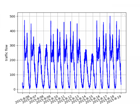
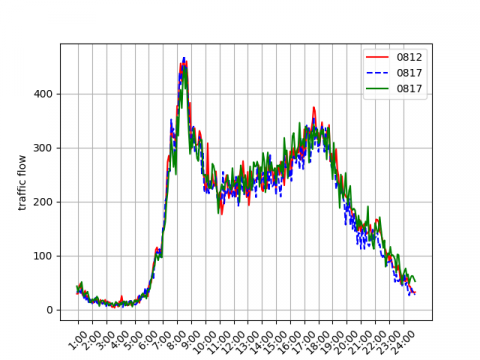
Use historical trend method and exponential smoothing method to repair data missed by fault of equipment [29]. Part of the experimental data after repairing as shown in Figure 4. As the Figure 4a shows, the experimental data has obvious continuity, periodicity, and tidal nature. As the Figure 4b shows, daily peak of traffic flow is from 7:00 to 9:00 and from 16:00 to 19:00.
(a) Data from August 6 to 19 at station ID 1027
(b) Data of three days at station ID 1027
Figure 4. Part of the experimental data
5.2 Experimental environment and related parameter
We verify SPGAPSO-CKRVM with an 8-node Spark cluster built by virtual machines. The cluster includes CentOS-6.10-x64, Spark2.1.1-bin-hadoop2.7, hadoop-2.7.2.tar, pyspark-2.3.2 and py4j-0.10.8.1. The parameters of SPGAPSO-CKRVM are shown in Table 1.
Table 1. The parameters of SPGAPSO-CKRVM
|
Parameter |
Value |
|
Population size Maximum times of iterations Minimum fitness Crossover rate Mutation rate Learning factor Particle velocity Particle position |
10 20 10−5 0.6 0.2 1.5 [-0.2,0.2] [-8,8] |
5.3 Experimental results analysis
Because traffic congestion, travel delay, and road accidents mostly occur in daily peak of traffic flow, predicting the traffic flow in daily peak is more meaningful than predicting the traffic flow in other time [30-32]. For traffic flow prediction, a kernel function which predicts traffic flow in daily peak accurately should be considered to have greater performance. First, we use accuracy (i.e. 1-MAPE) to verify kernel function performance. In addition, we define Peak Hour Accuracy (PHA) (i.e. accuracy of predicting traffic flow from 7:00 to 9:00 and from 16:00 to 19:00) to verify kernel function performance. The experimental results are shown in Table 2.
Because the traffic data of ramp is more random and difficult to predict than the traffic data of general road, the accuracy of all kernel functions on Sections 1 and Sections 2 are greater than that of Sections 3. As shown in Table 2, the performance of combined kernel functions (i.e. No.5 and No.6 kernel functions) are generally better than the performance of the single kernel functions (i.e. kernel functions from No.1 to No.4.). Except in Sections 1, the accuracy of No.6 kernel function is always greater than that of No.5 kernel function. In all Sections, PHA of No.6 kernel function is always greater than that of No.5 kernel function. Therefore, we use No.6 kernel function as the kernel function of RVM for subsequent experiments.
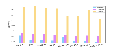
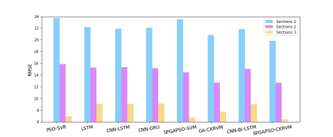
Different prediction models based on machine learning and deep learning, namely the proposed SPGAPSO-CKRVM, SPGAPSO-SVM, GA-CKRVM, PSO-SVR, LSTM, CNN-LSTM, CNN-GRU, CNN-Bi-LSTM were applied herein. Where, SPGAPSO-SVM represents SVM optimized by the same parameter optimization algorithm as SPGAPSO-CKRVM. GA-CKRVM represents RVM based on combined kernel function optimized by GA. PSO-SVR represents a model based on SVM optimized by PSO. CNN-GRU represents a deep model based on CNN and GRU. Table 3 lists the RMSE, MAE and MAPE for the different prediction models.
As shown in Table 3, PSO-SVR has the worst performance. Deep learning models based on RNN such as LSTM, CNN-LSTM, CNN-GRU and CNN-Bi-LSTM are significantly better than models based on SVM. SPGAPSO-SVM and GA-CKRVM are slightly better than the above models in certain sections. In all sections, SPGAPSO-CKRVM is always superior to other comparison models. Figure 5 clearly illustrate MAPE and RMSE of the various prediction models on different traffic sections.
Table 2. Experimental results of kernel function performance
|
NO. |
kernel function |
Sections 1 |
Sections 2 |
Sections 3 |
|||
|
Accuracy |
PHA |
Accuracy |
PHA |
Accuracy |
PHA |
||
|
1 |
$\exp \left(-\frac{\left\|x-x_{i}\right\|}{2 \sigma^{2}}\right)$ |
0.8084 |
0.8717 |
0.7964 |
0.8576 |
0.7131 |
0.8187 |
|
2 |
$\exp \left(-\frac{\left\|x-x_{i}\right\|^{2}}{2 \sigma^{2}}\right)$ |
0.8520 |
0.9292 |
0.8355 |
0.9057 |
0.7452 |
0.8515 |
|
3 |
$x^{T} x_{i}$ |
0.8529 |
0.9282 |
0.8310 |
0.9011 |
0.7472 |
0.8508 |
|
4 |
$\gamma\left(x x_{i}+1\right)^{d}+c$ |
0.8514 |
0.9272 |
0.8367 |
0.9056 |
0.7544 |
0.8502 |
|
5 |
$\exp \left(-\frac{\left\|x-x_{i}\right\|}{2 \sigma^{2}}\right) \lambda+(1-\lambda)\left[\gamma\left(x x_{i}+1\right)^{d}+c\right]$ |
0.8529 |
0.9301 |
0.8368 |
0.9059 |
0.7554 |
0.8521 |
|
6 |
$\exp \left(-\frac{\left\|x-x_{i}\right\|^{2}}{2 \sigma^{2}}\right) \lambda+(1-\lambda)\left[\gamma\left(x x_{i}+1\right)^{d}+c\right]$ |
0.8535 |
0.9333 |
0.8387 |
0.9061 |
0.7555 |
0.8538 |
Table 3. Experimental results of algorithm accuracy
|
Algorithm |
Sections 1 |
Sections 2 |
Sections 3 |
||||||
|
MSE |
RMSE |
MAPE |
MSE |
RMSE |
MAPE |
MSE |
RMSE |
MAPE |
|
|
PSO-SVR [33] |
564.06 |
23.75 |
0.1624 |
251.54 |
15.86 |
0.1724 |
48.86 |
6.99 |
0.2701 |
|
LSTM |
493.13 |
22.21 |
0.1435 |
234.37 |
15.31 |
0.1689 |
82.88 |
9.10 |
0.2702 |
|
CNN-LSTM [15] |
483.18 |
21.92 |
0.1438 |
235.89 |
15.36 |
0.1663 |
82.43 |
9.08 |
0.2659 |
|
CNN-GRU [34] |
487.46 |
22.07 |
0.1429 |
229.62 |
15.15 |
0.1648 |
84.10 |
9.17 |
0.2852 |
|
SPGAPSO-SVM |
551 |
23.47 |
0.1577 |
210 |
14.49 |
0.1638 |
45.08 |
6.71 |
0.2368 |
|
GA-CKRVM [23] |
433.53 |
20.82 |
0.1412 |
161.56 |
12.71 |
0.1616 |
62.24 |
7.76 |
0.2347 |
|
CNN-Bi-LSTM [16] |
477.35 |
21.84 |
0.1396 |
227.11 |
15.07 |
0.1622 |
81.79 |
9.04 |
0.2600 |
|
SPGAPSO-CKRVM |
392.43 |
19.81 |
0.1383 |
161.1 |
12.69 |
0.1589 |
41.09 |
6.41 |
0.2232 |
(a) MAPE of various prediction models
(b) RMSE of various prediction models
Figure 5. Experimental results of algorithm accuracy
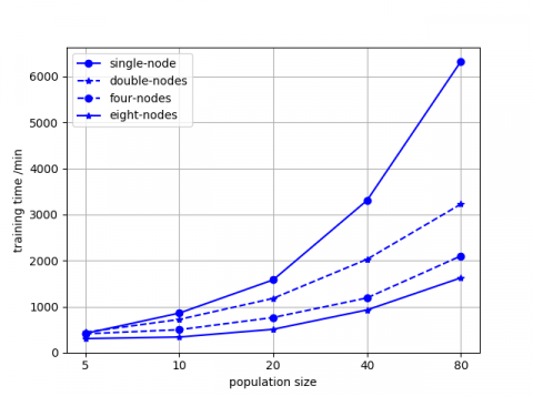
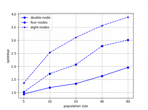
The experiment of algorithm scalability is used to test whether it is possible to increase the algorithm efficiency by adding additional nodes. We calculate speedup to evaluate the effect of parallelization. Run SPGAPSO-CKRVM ten times based on a single node, double nodes, four nodes and eight nodes respectively. Record the experimental results and calculate speedup of SPGAPSO-CKRVM. Speedup defined as follows:
$S_{n}=\frac{T_{1}}{T_{n}}$ (22)
where, T1 is sequential calculation time of model. Tn is parallel calculation time of model based on n nodes. Ideally, speedup is equal to the number of nodes. The experimental results are shown in Figure 6.
Population size determines the calculation of SPGAPSO-CKRVM. As the Figure 6a shows, the training time of SPGAPSO-CKRVM increases linearly with the calculation increasing gradually. The gap of training time of SPGAPSO-CKRVM based on different number of nodes is small when the calculation is little. As the calculation increasing, the training time of SPGAPSO-CKRVM based on eight-nodes is much lower than the training time of SPGAPSO-CKRVM based on four-nodes, double-nodes and single-node. The reason is that each calculation node is responsible for few calculations when the number of calculation nodes is large.
As the Figure 6b shows, the acceleration effect of the cluster is not obvious when the calculation is little. The reason is that the basic operations such as starting cluster, dividing tasks and allocating resources of the cluster are time-consuming. At this moment, the cluster has not achieved deserved effect. As the calculation increasing, the advantages of parallel calculation are becoming more and more obvious. The speedup is increasing and approaching gradually the ideal value. The experimental results verify that SPGAPSO-CKRVM proposed in this paper has good scalability.
(a) Training time of SPGAPSO-CKRVM with different number of nodes
(b) Speedup of SPGAPSO-CKRVM with different number of nodes
Figure 6. Experiment results of algorithm scalability
To construct a prediction model for traffic flow, RVM based on a combined kernel function and heuristic algorithms were employed. Parameter optimization algorithm of RVM was parallelized by Spark. SPGAPSO-CKRVM is proposed. The real data of Whitemud Drive in Canada were utilized to verify the prediction model. Experimental results show that the model called on SPGAPSO-CKRVM is superior to other methods in accuracy. In addition, SPGAPSO-CKRVM has less time consumption of parameter optimization than other models. Further research will include:
• Consider more factors affecting traffic flow such as average speed, lane occupancy rate and traffic flow on the adjacent roads.
• We use the original GA and PSO in this paper. For parameter optimization of RVM, most of heuristic algorithms have the problem that the convergence speed is too fast in early period of iterations, which leads to decrease of the population diversity in later period of iterations. In further research, we will try to combine RVM with complex heuristic algorithms such as Adaptive Genetic Algorithm (AGA) and Quantum Particle Swarm Algorithm (QPSO).
• Although the testing speed of RVM is extremely fast, the training speed is not ideal. We will use parallelization techniques to reduce training time of RVM.
• We will research the combination of RVM and deep learning algorithms. Deep learning algorithms such as DBN and CNN are used to extract traffic data features and RVM is used to predict traffic flow to construct a deep prediction model.
This work is supported by the Inner Mongolia Key Technological Development Program (Grant No.: 2019ZD015) and the Key Scientific and Technological Research Program of Inner Mongolia Autonomous Region (Grant No.: 2019GG273). The authors thank Dr. Jianxiong Wan for revising his English expressions.
[1] Makino, H., Tamada, K., Sakai, K., Kamijo, S. (2018). Solutions for urban traffic issues by ITS technologies. IATSS Research, 42(2): 49-60. https://doi.org/10.1016/j.iatssr.2018.05.003
[2] Kistan, T., Gardi, A., Sabatini, R., Ramasamy, S., Batuwangala, E. (2017). An evolutionary outlook of air traffic flow management techniques. Progress in Aerospace Sciences, 88: 15-42. https://doi.org/10.1016/j.paerosci.2016.10.001
[3] Singh, S.K., Saraswat, A. (2019). Design service volume, capacity, level of service calculation and forecasting for a semi-urban city. Revue d'Intelligence Artificielle, 33(2): 139-143. https://doi.org/10.18280/ria.330209
[4] Lin, H., Li, L.X., Wang, H. (2020). A survey on research and application of support vector machines in ITS. Journal of Frontiers of Computer Science and Technology, 14(6): 901-917. http://fcst.ceaj.org/EN/Y2020/V14/I6/901
[5] Nagy, A.M., Simon, V. (2018). Survey on traffic prediction in smart cities. Pervasive and Mobile Computing, 50: 148-163.
[6] Ding, A., Zhao, X., Jiao, L. (2002). Traffic flow time series prediction based on statistics learning theory. In Proceedings. The IEEE 5th International Conference on Intelligent Transportation Systems, pp. 727-730. https://doi.org/10.1109/ITSC.2002.1041308
[7] Tipping, M.E. (2001). Sparse Bayesian learning and the relevance vector machine. Journal of Machine Learning Research, 1: 211-244.
[8] Zhao, C., Zhang, Y. (2012). Research progress and analysis on methods for classification of RVM. CAAI Transactions on Intelligent Systems, 7(4): 294-301.
[9] Tan, M.C., Wong, S.C., Xu, J.M., Guan, Z.R., Zhang, P. (2009). An aggregation approach to short-term traffic flow prediction. IEEE Transactions on Intelligent Transportation Systems, 10(1): 60-69. https://doi.org/10.1109/TITS.2008.2011693
[10] Cao, J., Zhang, M.Y. (2011). Detection and estimation for the traffic flow based on Kalman filter. Journal of Beijing Institute of Technology, 20(5): 271-275.
[11] Cao, C., Xu, J. (2007). Short-term traffic flow predication based on PSO-SVM. In International Conference on Transportation Engineering, pp. 167-172. https://doi.org/10.1061/40932(246)28
[12] Tian, Y., Zhang, K., Li, J., Lin, X., Yang, B. (2018). LSTM-based traffic flow prediction with missing data. Neurocomputing, 318: 297-305. https://doi.org/10.1016/j.neucom.2018.08.067
[13] Fu, R., Zhang, Z., Li, L. (2016). Using LSTM and GRU neural network methods for traffic flow prediction. In 2016 31st Youth Academic Annual Conference of Chinese Association of Automation (YAC), pp. 324-328. https://doi.org/10.1109/YAC.2016.7804912
[14] Duan, Z., Yang, Y., Zhang, K., Ni, Y., Bajgain, S. (2018). Improved deep hybrid networks for urban traffic flow prediction using trajectory data. IEEE Access, 6: 31820-31827. https://doi.org/10.1109/ACCESS.2018.2845863
[15] Liu, Q., Wang, B., Zhu, Y. (2018). Short‐term traffic speed forecasting based on attention convolutional neural network for arterials. Computer-Aided Civil and Infrastructure Engineering, 33(11): 999-1016. https://doi.org/10.1111/mice.12417
[16] Liu, Y., Zheng, H., Feng, X., Chen, Z. (2017). Short-term traffic flow prediction with Conv-LSTM. In 2017 9th International Conference on Wireless Communications and Signal Processing (WCSP), pp. 1-6. https://doi.org/10.1109/WCSP.2017.8171119
[17] Jin, X., Hui, X.F. (2012). Financial assets price prediction based on relevance vector machine with genetic algorithm. JCIT: Journal of Convergence Information Technology, 7(5): 90-96. https://doi.org/10.4156/jcit.vol7.issue5.12
[18] Shen, Z., Wang, W., Shen, Q., Li, Z. (2017). Hybrid CSA optimization with seasonal RVR in traffic flow forecasting. TIIS, 11(10): 4887-4907.
[19] Shen, Z., Wang, W., Shen, Q., Zhu, S., Fardoun, H.M., Lou, J. (2020). A novel learning method for multi-intersections aware traffic flow forecasting. Neurocomputing, 398: 477-484. https://doi.org/10.1016/j.neucom.2019.04.094
[20] Wu, Y.W., Ning, Q. (2017). Distributed SVM parameter optimization based on Hadoop. Computer Engineering and Science, 39(6): 1042-1047.
[21] Li, K., Li, P., Lu, Y.J., Zhang, G.P., Huang, Y.H. (2016). The parallel algorithms for LIBSVM parameter optimization based on Spark. Journal of Nanjing University (Natural Sciences), 52(2): 343-352.
[22] MacKay, D.J. (1992). Bayesian interpolation. Neural Computation, 4(3): 415-447. https://doi.org/10.1162/neco.1992.4.3.415
[23] Bing, Q., Gong, B., Yang, Z., Shang, Q., Zhou, X. (2015). Short-term traffic flow local prediction based on combined kernel function relevance vector machine model. Mathematical Problems in Engineering, 154703. https://doi.org/10.1155/2015/154703
[24] Xing, Y., Ban, X., Guo, C. (2017). Probabilistic forecasting of traffic flow using multikernel based extreme learning machine. Scientific Programming, 2073680. https://doi.org/10.1155/2017/2073680
[25] Zhang, L., Alharbe, N. R., Luo, G., Yao, Z., Li, Y. (2018). A hybrid forecasting framework based on support vector regression with a modified genetic algorithm and a random forest for traffic flow prediction. Tsinghua Science and Technology, 23(4): 479-492. https://doi.org/10.26599/TST.2018.9010045
[26] Li, Z., Xiong, W., Yuan, X., Zou, X. (2019). A short-term photovoltaic output prediction method based on improved PSO-RVM algorithm. In 2019 IEEE 10th International Symposium on Power Electronics for Distributed Generation Systems (PEDG), pp. 384-389. https://doi.org/10.1109/PEDG.2019.8807621
[27] Zaharia, M., Chowdhury, M., Franklin, M.J., Shenker, S., Stoica, I. (2010). Spark: Cluster computing with working sets. HotCloud, 10: 1-7.
[28] Zaharia, M., Chowdhury, M., Das, T., Dave, A., Ma, J., McCauly, M., Stoica, I. (2012). Resilient distributed datasets: A fault-tolerant abstraction for in-memory cluster computing. In Presented as part of the 9th {USENIX} Symposium on Networked Systems Design and Implementation ({NSDI} 12), pp. 15-28.
[29] Smith, B.L., Scherer, W.T., Conklin, J.H. (2003). Exploring imputation techniques for missing data in transportation management systems. Transportation Research Record, 1836(1): 132-142. https://doi.org/10.3141%2F1836-17
[30] Hao, W., Kamga, C., Wan, D. (2016). The effect of time of day on driver's injury severity at highway-rail grade crossings in the United States. Journal of Traffic and Transportation Engineering (English Edition), 3(1): 37-50. https://doi.org/10.1016/j.jtte.2015.10.006
[31] Arhin, S., Noel, E., Anderson, M.F., Williams, L., Ribisso, A., Stinson, R. (2016). Optimization of transit total bus stop time models. Journal of Traffic and Transportation Engineering (English Edition), 3(2): 146-153. https://doi.org/10.1016/j.jtte.2015.07.001
[32] Jin, S., Hou, Z., Chi, R., Bu, X. (2016). Model free adaptive predictive control approach for phase splits of urban traffic network. In 2016 Chinese Control and Decision Conference (CCDC), pp. 5750-5754. https://doi.org/10.1109/CCDC.2016.7532027
[33] Cao, C., Xu, J. (2007). Short-term traffic flow predication based on PSO-SVM. In International Conference on Transportation Engineering, pp. 167-172. https://doi.org/10.1061/40932(246)28
[34] Du, S., Li, T., Gong, X., Horng, S.J. (2018). A hybrid method for traffic flow forecasting using multimodal deep learning. International Journal of Computational Intelligence Systems, 13(2): 85-97. https://arxiv.org/abs/1803.02099