Ibrahim Chouidira* | Djalal Eddine Khodja | Salim Chakroune
OPEN ACCESS
The objective of this study is to present artificial intelligence (AI) technique for detection and localization of fault in induction machine fault, through a multi-winding model for the simulation of four adjacent broken bars and three-phase model for the simulation of short-circuit between turns. In this work, it was found that the application of artificial neural networks (ANN) based on Root mean square values (RMS) plays a big role for fault detection and localization. The simulation and obtained results indicate that ANN is able to detect the faulty with high accuracy.
Induction machine, faults detection and localization, broken bars, artificial neural network (ANN), root mean square (RMS), multi winding, three-phase model
With the advantages of induction machine especially in durability and cost, it has recently become the most widely used in the field of control systems with fault detection and diagnosis. Studies in this area have evolved considerably in order to avoid recurrent malfunctions that occur in the machine. Thus, no control system is safe from failure. Therefore, it is very important to pre-detect the various defects that may occur in these systems through the use of traditional or modern methods that allow us to monitor and control by taking preventive action to detect these incidents sudden accidents on the machine [1].
The diagnosis of stator turns short-circuit faults and broken bars at rotor level during the operation of induction machine is assignment difficult. Thus the major problem is connected how to detect faults. Therefore, early detection of turns short-circuits and broken bars during machine operation would remove following harm to adjacent coils and the stator and bearing at rotor [2, 3]. In this context, during the last two decades, the fault diagnosis of in asynchronous machine has turn on interest great from researchers. Main research has been executed for the development of various techniques and methods for fault detection and diagnosis. It has proposed an algorithm for the online detection of rotor bar breakage in induction motors based on the use of wavelet packet decomposition and neural networks [4]. A new set of feature coefficients is obtained by the WPD of the stator current, during used to build a neural network for fault detection, so thus accurately differentiates between healthy and faulty conditions. The algorithm analyzes rotor bar faults by WPD of the induction motor stator current. Whereas Seera et al., [5] suggest the insert a novel approach to detect and classify comprehensive fault conditions of induction motors using a hybrid fuzzy min–max (FMM) neural network and classification and regression tree (CART) is proposed based on MCSA technique used for stator-current signal acquisition, where by the motor current signature analysis method is applied to form a database comprising stator current signatures under different motor conditions. Among the works for turns in short-circuit for detection and locate faults is the work [6, 7] Bouzid et al., and Dash, et al., present the importance of using a technique neural network (NN) by a feed forward multilayer-perceptron trained by back propagation. While Zidani et al. [8], which proposes the problem of detection and diagnosis of induction motor faults introducing the fuzzy logic strategy, based on the stator current Concordia patterns on and a better understanding of heuristics underlying the motor faults detection and diagnosis.
To solve these defects, this paper establishes a tow model based on a multi-winding and three-phase, to simulate broken bars and turns in short-circuit, with the aim faults diagnosis at an early stage. The findings extraction gives light new to the application of neural networks based on RMS to facilitate detection and localization.
This paper is organized as follows: Section 1 introduces two models multi-winding and three-phase, Section 2 describes the way neural networks work by dependence on RMS values. Finally, we present the obtained results and verification of induction machine behavior using artificial neural networks (ANN).
To generate the healthy and faulty states, we use two models: multi winding and three-phase of induction machine. As described below.
2.1 Multi winding model
The equations of model fault of induction motor can be written as [9, 10]:
$[\mathrm{L}] \frac{\mathrm{d} \mathrm{l}}{\mathrm{d} \mathrm{t}}=[\mathrm{V}]-[\mathrm{R}][1]$ (1)
$\left[\begin{array}{ccccc}{\mathrm{L}_{\mathrm{sc}}} & {0} & {-\mathrm{N}_{\mathrm{r}} \mathrm{M}_{\mathrm{sr}} / 2} & {0} & {0} \\ {0} & {\mathrm{L}_{\mathrm{sc}}} & {0} & {\mathrm{N}_{\mathrm{r}} \mathrm{M}_{\mathrm{sr}} / 2} & {0} \\ {-3 \mathrm{M}_{\mathrm{sr}} / 2} & {0} & {\mathrm{L}_{\mathrm{rc}}} & {0} & {0} \\ {0} & {3 \mathrm{M}_{\mathrm{sr}} / 2} & {0} & {\mathrm{L}_{\mathrm{rc}}} & {0} \\ {0} & {0} & {0} & {0} & {\mathrm{L}_{\mathrm{e}}}\end{array}\right] \frac{\mathrm{d}}{\mathrm{d} t}\left[\begin{array}{l}{\mathrm{I}_{\mathrm{ds}}} \\ {\mathrm{I}_{\mathrm{qs}}} \\ {\mathrm{I}_{\mathrm{dr}}} \\ {\mathrm{I}_{\mathrm{qr}}} \\ {\mathrm{I}_{\mathrm{e}}}\end{array}\right]=\left[\begin{array}{c}{V_{\mathrm{ds}}} \\ {\mathrm{V}_{\mathrm{qs}}} \\ {0} \\ {0} \\ {0}\end{array}\right]-$ $\left[\begin{array}{ccccc}{\mathrm{R}_{\mathrm{s}}} & {-\mathrm{L}_{\mathrm{sc}} \omega_{\mathrm{r}}} & {0} & {\mathrm{N}_{\mathrm{r}} M_{\mathrm{sr}} \omega_{\mathrm{r}} / 2} & {0} \\ {\mathrm{L}_{\mathrm{sc}} \omega_{\mathrm{r}}} & {\mathrm{R}_{\mathrm{s}}} & {\mathrm{N}_{\mathrm{r}} \mathrm{M}_{\mathrm{sr}} \omega_{\mathrm{r}} / 2} & {0} & {0} \\ {0} & {0} & {\mathrm{R}_{\mathrm{r}}} & {0} & {0} \\ {0} & {0} & {0} & {\mathrm{R}_{\mathrm{r}}} & {0} \\ {0} & {0} & {0} & {0} & {\mathrm{R}_{\mathrm{e}}}\end{array}\right]\left[\begin{array}{l}{\mathrm{I}_{\mathrm{ds}}} \\ {\mathrm{I}_{\mathrm{qs}}} \\ {\mathrm{I}_{\mathrm{dr}}} \\ {\mathrm{I}_{\mathrm{qr}}} \\ {\mathrm{I}_{\mathrm{e}}}\end{array}\right]$
With defect model of the rotor in order to simulate the defect of rotor broken bars, a fault resistance RRF is given:
$\left[\mathrm{R}_{\mathrm{RF}}\right]=\left[\mathrm{R}_{\mathrm{R}}\right]+\left[\begin{array}{ccccccc}{0} & {\cdots} & {0} & {0} & {0} & {\cdots} & {\cdots} \\ {\vdots} & {\ldots} & {\vdots} & {\vdots} & {\vdots} & {\vdots} & {\cdots} \\ {0} & {\cdots} & {0} & {0} & {0} & {0} & {\cdots} \\ {0} & {\cdots} & {0} & {\mathrm{R}_{\mathrm{bk}}} & {-\mathrm{R}_{\mathrm{bk}}} & {0} & {\cdots} \\ {0} & {\cdots} & {0} & {-\mathrm{R}_{\mathrm{bk}}} & {\mathrm{R}_{\mathrm{bk}}} & {0} & {\cdots} \\ {0} & {\cdots} & {0} & {0} & {0} & {0} & {\cdots} \\ {\vdots} & {\cdots} & {\vdots} & {\vdots} & {\vdots} & {\cdots}\end{array}\right]$
where, the four terms of this matrix are [11, 12]:
$\begin{aligned} \mathrm{R}_{\mathrm{rdd}}=& 2 \mathrm{R}_{\mathrm{b}}(1-\cos (\mathrm{a}))+2 \frac{\mathrm{R}_{\mathrm{e}}}{\mathrm{N}_{\mathrm{r}}}+\frac{2}{\mathrm{N}_{\mathrm{r}}}(1-\cos (\mathrm{a})) \sum_{\mathrm{k}} \mathrm{R}_{\mathrm{bkf}}(1-\cos (2 \mathrm{k}-1) \mathrm{a}) \end{aligned}$ (2)
$\left.\mathbf{R}_{\mathrm{rdq}}=-\frac{2}{\mathrm{N}_{\mathrm{r}}}(\mathbf{1}-\cos (\mathbf{a})) \sum_{\mathbf{k}} \mathbf{R}_{\mathrm{bkf}} \sin (2 \mathbf{k}-\mathbf{1}) \mathbf{a}\right)$ (3)
$\mathbf{R}_{\mathrm{rqd}}=-\frac{2}{\mathrm{N}_{\mathrm{r}}}(\mathbf{1}-\mathbf{c o s}(\mathbf{a})) \sum_{\mathbf{k}} \mathbf{R}_{\mathrm{bkf}} \sin (2 \mathbf{k}-\mathbf{1})$a) (4)
And
$\begin{aligned} \mathrm{R}_{\mathrm{rqq}}=2 \mathrm{R}_{\mathrm{b}}(1-\cos (\mathrm{a})) &+2 \frac{\mathrm{R}_{\mathrm{e}}}{\mathrm{N}_{\mathrm{r}}} +\frac{2}{\mathrm{N}_{\mathrm{r}}}(1-\cos (\mathrm{a})) \sum_{\mathrm{k}} \mathrm{R}_{\mathrm{bkf}}(1+\cos (2 \mathrm{k}-1) \mathrm{a}) \end{aligned}$
2.2 Three-phase model
Another method for modeling of the induction machine is presented. The defects of short-circuit between coils, taking into account the changing parameters such as resistors and inductors based on the classics assumptions. The machine can be modeled by the following equations [13]:
$\left[\mathrm{V}_{\mathrm{s}}\right]=\left[\mathrm{R}_{\mathrm{s}}\right]\left[\mathrm{I}_{\mathrm{s}}\right]+\frac{\mathrm{d}}{\mathrm{dt}}\left[\Phi_{\mathrm{s}}\right]$ (5)
$[0]=\left[\mathrm{R}_{\mathrm{r}}\right]\left[\mathrm{I}_{\mathrm{r}}\right]+\frac{\mathrm{d}}{\mathrm{dt}}\left[\Phi_{\mathrm{r}}\right]$ (6)
$\left.\left[\Phi_{s}\right]=\left(\left[M_{s s}\right]+\left[L_{s}\right]\right)\left[I_{s}\right]+\left[M_{s r}\right]\left[I_{r}\right]\right)$ (7)
$\left[\Phi_{r}\right]=\left[M_{r s}\right]\left[I_{s}\right]+\left(\left[M_{r r}\right]+\left[L_{r}\right]\right)\left[I_{r}\right]$ (8)
The following matrices represent voltages, currents, and fluxes at the stator:
$\left[V_{s}\right]=\left[\begin{array}{c}{V_{s a}} \\ {V_{s b}} \\ {V_{s c}}\end{array}\right] ;\left[I_{s}\right]=\left[\begin{array}{c}{I_{s a}} \\ {I_{s b}} \\ {I_{s c}}\end{array}\right] ;\left[\Phi_{s}\right]=\left[\begin{array}{c}{\Phi_{s a}} \\ {\Phi_{s b}} \\ {\Phi_{s c}}\end{array}\right]$
The matrices represent voltages, currents, and fluxes at the rotor, the coefficients of short–circuit as following:
Short-circuit coefficient relative to the 1st stator phase:
$K_{s a}=\frac{N_{c c 1}}{N_{s}}$
Short-circuit coefficient relative to the 2nd stator phase:
$K_{s b}=\frac{N_{c c 2}}{N_{s}}$
Short-circuit coefficient relative to the 3nd stator phase:
$K_{s c}=\frac{N_{c c 3}}{N_{s}}$
With Ncc: The number of turns in short-circuit.
The number of useful turns for the three stator phases, is then given by:
$N_{1}=N_{s}-N_{c c 1}=\left(1-K_{s a}\right) N_{s}=f_{s a} N_{s}$
$N_{2}=N_{s}-N_{c c 2}=\left(1-K_{s b}\right) N_{s}=f_{s b} N_{s}$
$N_{3}=N_{s}-N_{c c 3}=\left(1-K_{s c}\right) N_{s}=f_{s c} N_{s}$
The matrixes $\left[R_{S}\right],\left[L_{s f}\right],\left[M_{s s}\right],\left[M_{s r}\right],\left[M_{r s}\right]$ depend of three coefficient $f_{s a}, f_{s b}, f_{s c}$ are given by the following terms:
$\left[L_{s f}\right]=\left[\begin{array}{ccc}{f_{s a}^{2} L_{s f}} & {0} & {0} \\ {0} & {f_{s a}^{2} L_{s f}} & {0} \\ {0} & {0} & {f_{s a}^{2} L_{s f}}\end{array}\right]$ (9)
$\left[M_{s s}\right]=M_{s}\left[\begin{array}{ccc}{f_{s a}^{2}} & {-\frac{f_{s a} f_{s b}}{2}} & {-\frac{f_{s a} f_{s c}}{2}} \\ {-\frac{f_{s a} f_{s b}}{2}} & {f_{s b}^{2}} & {-\frac{f_{s c} f_{s b}}{2}} \\ {-\frac{f_{s a} f_{s c}}{2}} & {-\frac{f_{s c} f_{s b}}{2}} & {f_{s c}^{2}}\end{array}\right]$ (10)
$\left[M_{s r}\right]=M\left[\begin{array}{ccc}{f_{s a} \cos \theta} & {f_{s a} \cos \left(\theta+\frac{2 \pi}{3}\right)} & {f_{s a} \cos \left(\theta-\frac{2 \pi}{3}\right)} \\ {f_{s b} \cos \left(\theta-\frac{2 \pi}{3}\right)} & {f_{s b} \cos \theta} & {f_{s b} \cos \left(\theta+\frac{2 \pi}{3}\right)} \\ {f_{s c} \cos \left(\theta+\frac{2 \pi}{3}\right)} & {f_{s c} \cos \left(\theta-\frac{2 \pi}{3}\right)} & {f_{s c} \cos \theta}\end{array}\right]$
With $\left[M_{s r}\right]=\left[M_{r s}\right]^{t}$
The matrix of stator resistances $\left[R_{s}\right]$ is given by:
$\left[R_{s}\right]=R s\left[\begin{array}{ccc}{f_{s a}} & {0} & {0} \\ {0} & {f_{s b}} & {0} \\ {0} & {0} & {f_{s c}}\end{array}\right]$ (11)
The set of rotor variables (flows and currents) can be changed to new variables with the same pulsation as the stator variables. Thus, all the parameters of the model will be independent of the angular position "θ" the transformation is given by the following matrix [14]
$[T]=\left[\begin{array}{ccc}{\cos \left(\theta+\frac{1}{2}\right)} & {\cos \left(\theta+\frac{2 \pi}{3}\right)+\frac{1}{2}} & {\cos \left(\theta-\frac{2 \pi}{3}\right)+\frac{1}{2}} \\ {\cos \left(\theta-\frac{2 \pi}{3}\right)+\frac{1}{2}} & {\cos \left(\theta+\frac{1}{2}\right)} & {\cos \left(\theta+\frac{2 \pi}{3}\right)+\frac{1}{2}} \\ {\cos \left(\theta+\frac{2 \pi}{3}\right)+\frac{1}{2}} & {\cos \left(\theta-\frac{2 \pi}{3}\right)+\frac{1}{2}} & {\cos \left(\theta+\frac{1}{2}\right)}\end{array}\right]$
It is easy to show that this matrix is orthogonal:
$[T]^{-1}=[T]^{T}$ (12)
Considering the Eq. (7) using the matrices T as:
$\left[\Phi_{s}\right]=\left[M_{s}\right]\left[I_{s}\right]+\left[M_{s r}\right]\left[I_{r}\right]\quad=\left[M_{s}\right]\left[I_{s}\right]+\left[M_{s r}\right][T]^{-1}[T]\left[I_{r}\right]$ (13)
When Simplify the equation written:
$\left[\Phi_{s}\right]=\left[M_{s}\right]\left[I_{s}\right]+\left[M_{s r}^{s}\right]\left[I_{r}^{s}\right]$ (14)
where,
$\left[M_{s r}^{s}\right]=\left[M_{s r}^{s}\right][T]^{-1}$ and $\left[I_{r}^{s}\right]=[T]\left[I_{r}\right]$
With:
$\left[M_{s r}^{s}\right]=\left[\begin{array}{ccc}{f_{s a} M} & {-f_{s a} \frac{M}{2}} & {-f_{s c} \frac{M}{2}} \\ {-f_{s b} \frac{M}{2}} & {f_{s b} M} & {-f_{s c} \frac{M}{2}} \\ {-f_{s c} \frac{M}{2}} & {-f_{s c} \frac{M}{2}} & {f_{s c} M}\end{array}\right]$ (15)
The global model of the induction machine in the presence of stator failures.
Flux equations:
$\frac{d \Phi_{r a}}{d t}=\delta\left(f_{s a} i_{s a}-\frac{f_{s b}}{2} i_{s b}-\frac{f_{s c}}{2} i_{s c}\right)-\frac{R_{r} A}{C} \Phi_{r a}-\left(\frac{R_{r} B}{c}+\frac{\sqrt{3}}{3} \omega_{r}\right) \Phi_{r b}-\left(\frac{R_{r} B}{c}+\frac{\sqrt{3}}{3} \omega_{r}\right) \Phi_{r c}$ (16)
$\begin{aligned} \frac{d \Phi_{r b}}{d t} &=\delta\left(-\frac{f_{s a}}{2} i_{s a}+f_{s b} i_{s b}-\frac{f_{s c}}{2} i_{s c}\right) \\-\left(\frac{R_{r} B}{c}+\frac{\sqrt{3}}{3} \omega_{r}\right) & \Phi_{r a}-\frac{R_{r} A}{c} \Phi_{r b}-\left(\frac{R_{r} B}{c}+\frac{\sqrt{3}}{3} \omega_{r}\right) \Phi_{r c} \end{aligned}$ (17)
$\begin{aligned} \frac{d \Phi_{r c}}{d t} &=\delta\left(-\frac{f_{s a}}{2} i_{s a}-\frac{f_{s b}}{2} i_{s b}+f_{s c} i_{s c}\right) -\left(\frac{R_{r} B}{c}+\frac{\sqrt{3}}{3} \omega_{r}\right) \Phi_{r a}-\left(\frac{R_{r} B}{c}+\frac{\sqrt{3}}{3} \omega_{r}\right) \Phi_{r b}-\frac{R_{r} A}{c} \Phi_{r c} \end{aligned}$ (18)
Stator current equations:
$\frac{d i_{s a}}{d t}=V_{S A}+K_{A 1} i_{s a}+K_{A 2} i_{s b}+K_{A 3} i_{s c}+K f_{s a} f_{s b}^{2} f_{s c}^{2}\left(G \Phi_{r a}+\left(\frac{\sqrt{3}}{2} \omega_{r}-\frac{G}{2}\right) \Phi_{r b}-\left(\frac{\sqrt{3}}{2} \omega_{r}-\frac{G}{2}\right) \Phi_{r c}\right)$ (19)
$\begin{aligned} \frac{d i_{s b}}{d t} &=V_{S B}+K_{B 1} i_{s a}+K_{B 2} i_{s b}+K_{B 3} i_{s c}+K f_{s a} f_{s b}^{2} f_{s c}^{2}\left(-\left(\frac{\sqrt{3}}{2} \omega_{r}-\frac{G}{2}\right) \Phi_{r a}+G \Phi_{r b}+\left(\frac{\sqrt{3}}{2} \omega_{r}-\frac{G}{2}\right) \Phi_{r c}\right) \end{aligned}$ (20)
$\frac{d i_{s c}}{d t}=V_{S C}+K_{C 1} i_{s a}+K_{C 2} i_{s b}+K_{C 3} i_{s c}+K f_{s a} f_{s b}^{2} f_{s c}^{2}\left(\left(\frac{\sqrt{3}}{2} \omega_{r}-\frac{G}{2}\right) \Phi_{r a}-\left(\frac{\sqrt{3}}{2} \omega_{r}+\frac{G}{2}\right) \Phi_{r b}+\Phi_{r c}\right)$ (21)
Used coefficients:
$V_{S A}=d_{1} f_{s a}^{2} f_{s c}^{2} u_{s a}+d_{2} f_{s a} f_{s b} f_{s c}^{2} u_{s b}+d_{2} f_{s a} f_{s b}^{2} f_{s c} u_{s c}$
$V_{S B}=d_{2} f_{s a} f_{s b} f_{s c}^{2} u_{s a}+d_{1} f_{s a}^{2} f_{s c}^{2} u_{s b}+d_{2} f_{s a}^{2} f_{s b} f_{s c} u_{s c}$
$V_{S A}=d_{2} f_{s a} f_{s b}^{2} f_{s c} u_{s a}+d_{2} f_{s a}^{2} f_{s b} f_{s c} u_{s b}+d_{1} f_{s a}^{2} f_{s b}^{2} u_{s c}$
$A=\left(l_{r f}+M_{r}\right)^{2}-\frac{M_{r}^{2}}{4} ; B=\frac{M_{r} l_{r f}}{2}+\frac{3 M_{r}^{2}}{4};$
$C=l_{r f}^{3}+3 l_{r f}^{2} M_{r}+\frac{9}{4} M_{r}^{2} l_{r f} ; \delta=\frac{M_{s r R}(A-B)}{c}; $
$T=\frac{M_{s r}^{2} R_{r}(A-B)^{2}}{c^{2}} ; z=M_{s r}-\frac{3 M_{s r}^{2} R_{r}(A-B)}{2 c};$
$\lambda=z+l_{s f} ; H=\lambda^{2}-\frac{z \lambda}{2}-\frac{z^{2}}{4}$
$\begin{aligned}|\Gamma| &=f_{s a}^{2} f_{s b}^{2} f_{s c}^{2}\left(\lambda^{3}-\frac{3 z^{2} \lambda}{2}-\frac{z^{3}}{4}\right) ; d_{1}=\left(z+l_{s f}\right)^{2}-\frac{z^{2}}{4} \\ d_{2} &=z\left(z+l_{s f}\right)^{2}+\frac{z^{2}}{4} ; K=\frac{M_{s r} H(A-B)}{c|\Gamma|} ; G=\frac{R_{r}(A-B)}{c} \end{aligned}$
$\left\{\begin{array}{l}{K_{A 1=}-\frac{3}{2}\left(d_{1}+d_{2}\right) T f_{s a}^{2} f_{s b}^{2} f_{s c}^{2}+R_{s} d_{1} f_{s a} f_{s b}^{2} f_{s c}^{2}} \\ {K_{A 2=}-\frac{3}{2} \frac{\left(d_{1}+3 d_{2}\right)}{2} T f_{s a} f_{s b}^{3} f_{s c}^{2}+R_{s} d_{2} f_{s a} f_{s b}^{2} f_{s c}^{2}} \\ {K_{A 3=}-\frac{3}{2} \frac{\left(d_{1}+3 d_{2}\right)}{2} T f_{s a} f_{s b}^{2} f_{s c}^{3}+R_{s} d_{2} f_{s a} f_{s b}^{2} f_{s c}^{2}} \\ {K_{B 1=}-\frac{3}{2} \frac{\left(d_{1}+3 d_{2}\right)}{2} T f_{s a}^{3} f_{s b} f_{s c}^{2}+R_{s} d_{2} f_{s a}^{2} f_{s b} f_{s c}^{2}} \\ {K_{B 2=}-\frac{3}{2}\left(d_{1}+d_{2}\right) T f_{s a}^{2} f_{s b}^{2} f_{s c}^{2}+R_{s} d_{1} f_{s a}^{2} f_{s b} f_{s c}^{2}} \\ {K_{B 3}=-\frac{3}{2} \frac{\left(d_{1}+3 d_{2}\right)}{2} T f_{s a}^{2} f_{s b} f_{s c}^{3}+R_{s} d_{2} f_{s a}^{2} f_{s b} f_{s c}^{2}}\\{K_{C 1=}-\frac{3}{2} \frac{\left(d_{1}+3 d_{2}\right)}{2} T f_{s a}^{3} f_{s b}^{2} f_{s c}+R_{s} d_{2} f_{s a}^{2} f_{s b}^{2} f_{s c}}\\{K_{C 2=}-\frac{3}{2} \frac{\left(d_{1}+3 d_{2}\right)}{2} T f_{s a}^{2} f_{s b}^{3} f_{s c}+R_{s} d_{2} f_{s a}^{2} f_{s b}^{2} f_{s c}}\\{K_{C 3=}-\frac{3}{2}\left(d_{1}+d_{2}\right) T f_{s a}^{2} f_{s b}^{2} f_{s c}^{2}+R_{s} d_{1} f_{s a}^{2} f_{s b}^{2} f_{s c}}\end{array}\right.$
The torque equation is given by:
$C_{e}=P \frac{M_{s r}}{L_{r}}\left[\left(I_{s b} \Phi_{r c}-I_{s c} \Phi_{r b}\right)-\left(I_{s a} \Phi_{r c}-I_{s c} \Phi_{r a}\right)+\right.\left.\left(I_{s a} \Phi_{r a}-I_{s b} \Phi_{r b}\right)\right]$
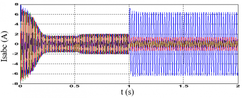
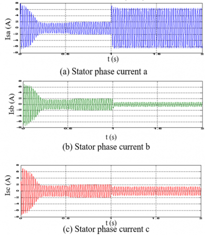
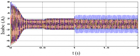
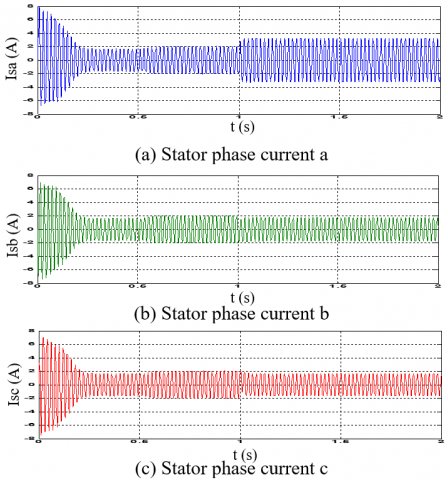
In this case, the more frequent bar breaks at the rotor level, we will present the rotor defects at the instant: t=1s break a bar, t=2s break two bars, t=3s break three bars, and t=4s break four bars, we apply a load of Cr=3.5Nm at t=0.5s, the value of the resistance of the broken bar will be considered equal to eleven (11) times, the value of the initial resistance. The currents of the stator phases are always out of phase by 120°. The modulation of the envelope of the stator current after the breaks of the bars is also noted, the increase of the amplitude of proportional to the number of broken bars which appears in the figures (1-2). With regard to the simulation of short-circuit faults between coils in an induction machine, in a first case, we presented the shapes of the stator currents in the case operation and with short-circuit-type faults between 40 turns (25%), and the second case we apply short circuit faults between 20 turns (12.5%). As shown in Figures (3-4 -5-6).
Figure 1. Stator current in case broken four bar
Figure 2. Stator phase current (a,b,c)
Figure 3. Stator current in case type short-circuit faults between 40 turns (25%)
Figure 4. Stator phase current (a,b,c) in case of short-circuit faults between 40 turns (25%)
Figure 5. Stator current in case of short-circuit faults between 20 turns (12.5%)
Figure 6. Stator phase current (a,b,c) in case of short-circuit faults between 20 turns (12.5%)
To application of neural networks to solve the problem of the diagnosis of failures of an electromechanical system, two major steps must be applied [15]:
• The first consists of studying the problem to be solved to validate its adaptability with a resolution by neural networks and define the objectives to be achieved in order to be able to control the quality of the chosen solution.
• The second is focused on the technique of neural network; it includes the choice of the type of network and its implementation (the type of learning and the number of hidden layers) depending on the characteristics of the problem studied and the objectives set.
The learning base of the ANN is put in the form of a file or table (matrix). The latter is represented by classes of vectors, where each class represents a type of operation, and each vector is represented by the effective values. In this case, each vector consists of 7 parameters (Ia, Ib, Ic, Va, Vb, Vc and w). These represent the input layer of the ANN. In fact, to go to the classification stage, for each we have parameters of 7 types of operation including normal operation.
Very rich databases (normal and abnormal operations), which have a lot of information about the defect. For this phase the following tasks have been realized:
• The machine was simulated in normal operation (healthy state);
• The machine has been simulated in abnormal mode (in the presence of defects: one broken bar, two bars, three bars, and four bars);
• The machine has been simulated in abnormal mode (in the presence of defects: short-circuit between 40 and 20 turns). The Table 1 shows the classification step that, we have got in case of healthy and faulty state.
Table 1. Classification of the several faults
|
Fault Type |
Symbol |
Code |
|||
|
|
|
S1 |
S2 |
S3 |
S4 |
|
Healthy state |
HS |
0 |
0 |
0 |
0 |
|
One broken bar |
BO |
1 |
0 |
0 |
0 |
|
Two broken bars |
BT |
0 |
1 |
0 |
0 |
|
Three Broken bars |
BTH |
0 |
0 |
1 |
0 |
|
Four broken bars |
BF |
0 |
0 |
0 |
1 |
|
Short circuit between 40 coils |
SCBT1 |
1 |
0 |
1 |
0 |
|
Short circuit between 20 coils |
SCBT2 |
1 |
1 |
0 |
0 |
For artificial neural networks (ANN) Block construction using multilayer perceptrons have been shown to be effective for form classification. The neural network we tested is multilayer network that use the back propagation algorithm for their learning. The purpose of this algorithm is to fit the synaptic weights so as to minimize the average value of the error on the set of drives. Therefore, the use of a layered neural network is preferable to try to solve the problem. The networks used are multi-layer networks, comprising an input layer that corresponds to the retina, an output layer that corresponds to the decision, and a number of so-called hidden layers. These hidden layers constitute the variables of internal representation of the problems. The network construction steps can be divided as follows:
• Choice of the inputs of the network, we use the effective values of the variables (Isa, Isb, Isc, Va, Vb, Vc and W) to determine the number of entries of the network (number of neurons of the hidden layer), which indicate that the number of entries in this network is equal to 7 variables
• Choice of the outputs, i.e. determination of the number of outputs and their nature, to facilitate the interpretation of the results of the output of the network by the expert system, our choice was oriented on the binary numbers (0,1) As the outputs are binary and the actual inputs, the output function will be a linear function and the activation function a sigmoid function.
• Determination of the number of hidden neurons and the number of hidden layers: they will be determined by trial and error from a learning algorithm. As illustrated in the following Figure 7:
Figure 7. Detection and localization defects by neural networks
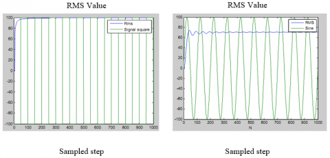
The effective value of a quantity is the square root of the sum of the squares of the constant term and the effective values of the various sinusoidal terms of the development in series:
$R M S=\sqrt{\frac{1}{t} \int_{0}^{t} u(t)^{2} d t}$ (23)
For a signal sampled by a sampling step Te. $u(t)^{2}$ will be known only at the sampling instants: $\int_{0}^{t} u(t)^{2} d t$ and can be approximated by the area between $u(t)^{2}$ discretized and the time axis.
For $\mathrm{N}$ samples: $\int_{0}^{t} u(t)^{2} d t \cong \sum_{i=0}^{N-1} u_{i}^{2} \times$ Te so: $R M S \cong\sqrt{\frac{1}{N \times T e} \sum_{i=0}^{N-1} u_{i}^{2} \times T e}$
$R M S \cong \sqrt{\frac{1}{N} \sum_{i=0}^{N-1} u_{i}^{2}}$
The results for the different types of input signals are detailed in the following graph, see Figure 8.
These graphs show the performance of the calculation method of RMS for square signal and sine signal.
Figure 8. Result of RMS calculation
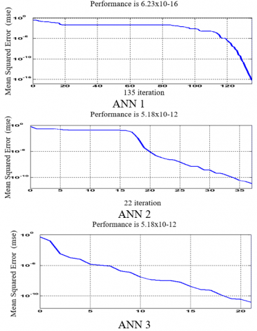
Neural network tests concern the verification of the performance of a network and its learning capacity. Once the network has been calculated, it is always necessary to carry out tests to verify that our network reacts correctly, the learning is a very important phase for the deployment of a neural network during which the behavior of the network is changed until the desired behavior is achieved In fact, these examples belong to two databases, the first one being the learning base and the second one being the test base of the neuron network on the case that belonged to the learning base of the neuron network the give better results and allows to estimate the generalization capacity of the network by evaluate types of functioning in case (healthy and defects) and the identified exactly by the three networks, this can be explained by the results obtained in the learning phase of the three networks (whose mean squared error values are close to zero). Regarding the test, the three networks on the examples are presented in the tables below.
Table 2. Test three networks
|
Number of neurons |
Entry layer |
Hidden layer |
Exit layer |
Mean square error |
|
ANN 1 |
7 |
8 |
4 |
6.23xe-16 |
|
ANN 2 |
7 |
7 |
4 |
5.18xe-12 |
|
ANN 3 |
7 |
6 |
4 |
9.64xe-12 |
Figure 9. Evaluation of the quadratic error as a function of the number of learning iterations
Note that the mean quadratic values of the networks studied are very close to zero, which means that the three neuron networks give better performance in the learning phase. At this phase we applied the defects at the rotor level (adjacent bar breakage) on ANN1 neuron networks and stator levels (short circuit between 40 and 20 turns) on ANN2 and ANN3 in several times as illustrated in the following tables:
Table 3. Application of the different defects
|
Application time |
Fault type |
|
|
ANN1 |
At t =1s |
Broken one bar |
|
At t =2s |
Broken two bar |
|
|
At t =3s |
Broken three bar |
|
|
At t =4s |
Broken four bar |
|
|
ANN2 |
At t =1s |
Short circuit between 40 turns |
|
ANN3 |
At t =1s |
Short circuit between 20 turns |
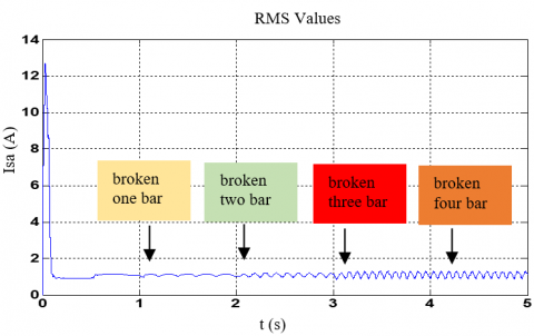
Figure 10. Evolution of the stator current and test of ANN1 in the case of four adjacent broken bars
For identify defects in a system, the diagnosis made by neural networks must have a sufficient number of examples during operation in a healthy case and defects to be able to learn, through the learning function, the examples are presented to the input network with the diagnostics corresponding to the output. After learning, the network not only recognizes the examples learned but also models resembling them, which corresponds to a certain robustness compared to signal deformations by the defect. When detecting a defect, the neural network ANN 1, present a change in Figure 10 at the moment of the application of the defect, for example, in time t=1s introduces first fault the outputs: S1, S2, S3, S4, respectively indicate the values: (1, 0, 0, 0) so the broken bar fault corresponding for other cases the outputs S1, S2, S3, S4 corresponding
• At t = 2 s represents (0, 1, 0, 0) break two bars;
• At t = 3 s represents (0, 0, 1, 0) three bar break;
• At t = 4 s represents (0, 0, 0, 1) four bar break.
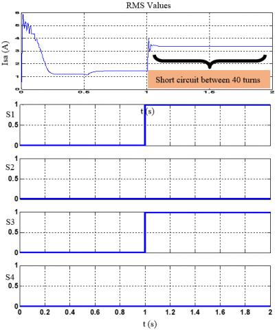
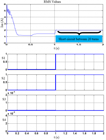
For the neuron network ANN 2and ANN 3 apply the fault at time t=1 s, we see that the graphs change in Figure 11 in the case of short circuit 40 and 20 turns, so this case the outputs: S1, S2, S3, S4, corresponding:
• At t = 1 s represents (1, 0, 1, 0) short circuit 40 turns;
• At t = 1 s represents (1, 1, 0, 0) short circuit 20turns.
Figure 11. Evolution of the stator current and test of the outputs of the second RNA2 and third RNA3 in the case of short-circuit 40 and 20 turns
The detection and early diagnosis allow reducing damage and maintaining other components of induction machine, through the study of defects influence and the behavior of the machine in case of operation fault. In this paper we presented the induction machine fault by using multi-winding model for simulation of broken bars and three-phase model for simulation of short- circuit between 20-40 turns. The new features are presented by multi layers neural network trained by retro-propagation algorithm. The RMS values of measured machine parameters are extracted by processing and monitoring of machine behavior in the presence of faults in order to obtain the indicators values
The proposed diagnosis method could be applied by artificial intelligence represented neural networks (ANN) on induction machine during several parametric studies (selection of the type of network, choice of inputs, and choice of outputs ...). With the data acquisition operation, this aims to establish the network learning base. To be reliable indicators for detection and location of fault broken bars and inter-turns short-circuit fault. These results clearly indicate that the proposed neural networks have a great importance for fault identification and capable to reduce the failure severity. Furthermore, it has been manifest that this approach is accurate and simple in the process implement diagnosis.
This work was supported by Electrical Engineering Laboratory (LGE), at the University of Mohamed Boudiaf- M’sila, (Algeria). We like to thank Dr. Djalal Eddine Khodja, and Dr. Salim Chakroune for their helps in the preparing of this paper.
Table 4. Appendix for simulation broken bar
|
Symbol |
Definition |
Value |
|
|
Pn |
output power |
1.1 |
kW |
|
Vs |
stator voltage per phase |
220 |
V |
|
Fs |
stator frequency |
50 |
Hz |
|
p |
poles pair number |
1 |
|
|
Rs |
stator resistance |
7.58 |
Ω |
|
Rr |
rotor resistance |
6.3 |
Ω |
|
Rb |
rotor bar resistance |
0.15 |
m Ω |
|
Re |
resistance of end ring segment |
0.15 |
m Ω |
|
Lb |
rotor bar inductance |
0.1 |
μH |
|
Le |
inductance of end ring |
0.1 |
μH |
|
Lsf |
leakage inductance of stator |
0.0265 |
H |
|
Nr |
number of rotor bars |
16 |
|
|
Ns |
number of turns per stator phase |
160 |
|
|
J |
moment of inertia |
0.0054 |
kg m2 |
|
e |
Air-gap mean diameter |
2 |
mm |
Table 5. Appendix for simulation short-circuit between coils
|
Symbol |
Definition |
Value |
|
|
Rs |
stator resistance |
1.633 |
Ω |
|
Rr |
rotor resistance |
0.93 |
Ω |
|
Lr |
inductance of rotor |
0.076 |
H |
|
Ls |
inductance of stator |
0.142 |
H |
|
J |
moment of inertia |
0.0111 |
kg m2 |
|
Ms |
mutual inductance stator nets |
0.099 |
H |
[1] Subotic, I., Dordevic, O., Gomm, B., Levi, E. (2019). Active and reactive power sharing between three-phase winding sets of a multiphase induction machine. IEEE Transactions on Energy Conversion, 34(3): 1401-1410. https://doi.org/10.1109/TEC.2019.2898545
[2] Benchabane, F., Guettaf, A., Yahia, K., Sahraoui, M. (2018). Experimental investigation on induction motors inter-turns short-circuit and broken rotor bars faults diagnosis through the discrete wavelet transform. e & i Elektrotechnik und Informationstechnik, 135(2): 187-194. https://doi.org/10.1007/s00502-018-0607-6
[3] Ojaghi, M., Sabouri, M., Faiz, J. (2018). Performance analysis of squirrel-cage induction motors under broken rotor bar and stator inter-turn fault conditions using analytical modeling. IEEE Transactions on Magnetics, 54(11): 1-5. https://doi.org/10.1109/tmag.2018.2842240
[4] Sadeghian, A., Ye, Z.M., Wu, B. (2009). Online detection of broken rotor bars in induction motors by wavelet packet decomposition and artificial neural networks. IEEE Trans. on Instrumentation and Measurement, 58(7): 187-194. https://doi.org/10.1109/TIM.2009.2013743
[5] Seera, M., Lee, C.P., Iahak, D., Singh, H. (2012). Fault detection and diagnosis of induction motors using motor current signature analysis and a hybrid FMM - CART model. IEEE Transactions on Neural Networks and Learning Systems, 23(1): 97-107. https://doi.org/10.1109/TNNLS.2011.2178443
[6] Bouzid, M., Champenois, G., Bellaaj, M., Signac, L., Jelassi, K. (2008). An effective neural approach for the automatic location of stator inter turn faults in induction motor. IEEE Transactions on Industrial Electronics, 55(12): 4277-4289. https://doi.org/10.1109/TIE.2008.2004667
[7] Dash, R.N., Subudhi, B. (2010). Stator inter-turn fault detection of an induction motor using neuro - fuzzy techniques. Archives of Control Sciences, 20(LVI3): 363-376. https://doi.org/10.2478/v10170-010-0022-7
[8] Zidani, F., El Hachemi Benbouzid, M., Diallo, D., Nait-Said, M.S. (2003). Induction motor stator faults diagnosis by a current Concordia pattern-based fuzzy decision system. IEEE Transactions on Energy Conversion, 18(4): 469-475. https://doi.org/10.1109/TEC.2003.815832
[9] Menacer, A., Nait-Said, M., Drid, S. (2004). Stator current analysis of incipient fault into asynchronous motor rotor bars using fourier fast transform. Journal of Electrical Engineering, 55(6): 122-130.
[10] Kechida, R., Menacer, A., Benakcha, A. (2010). Fault detection of broken rotor bars using stator current spectrum for the direct torque control induction motor. International Journal of Electrical and Computer Engineering, 4(6): 988-993.
[11] Menacer, A., Moreau, S., Benakcha, A., Nait-Said, M. (2006). Effect of the position and the number of broken bras on asynchronous motor stator current spectrum. EPE-Power Electronics and Motion Control, Portoroz, Slovenia, pp. 973-978.
[12] Djafar, D., Belhamdi, S. (2018). Speed control of induction motor with broken bars using sliding mode control (SMC) based to on Type-2 fuzzy logic controller (T2FLC). Advances in Modelling and Analysis C Journal, 73(4): 197-201. https://doi.org/10.18280/ama_c.730409
[13] Chen, S., Zivanovic, R. (2010). Modelling and simulation of stator and rotor fault conditions in induction machines for testing fault diagnostic techniques. European Transactions on Electrical Power, 20: 611-629.
[14] Khodja, D.E., Kheldoun, A. (2009). Three-phases model of the induction machine taking account the stator faults. International Science, 3(4): 124-127.
[15] Khodja, D.E., Chetate, B. (2008). ANN based double stator asynchronous machine diagnosis taking torque change into account. International Symposium on Power Electronics, Electrical Drives, Automation and Motion, 55(12): 1125-1129. https://doi.org/10.1109/speedham.2008.4581174