Xu Cheng | Chenyuan Zhao*
OPEN ACCESS
The accuracy of tourist flow prediction is crucial to the sustainable development of tourism industry. However, it is very difficult to forecast the highly nonlinear tourist flow in an accurate manner. The artificial neural network (ANN) has been widely adopted to predict nonlinear time series, but its shallow structure cannot effectively learn the features of high-dimensional tourist flow data. To solve the problem, this paper puts forward a tourist flow prediction model based on deep learning (DL). First, the deep belief network (DBN), with its strong ability to extract nonlinear features, was employed to extract effective features through unsupervised learning of historical tourist flow. Next, the echo state network (ESN) was effectively fused with the DBN. The ESN was placed at the top layer of the tourist flow prediction model, serving as the logic regression layer. Finally, the offline training and prediction effects of the proposed ESN-DBN were verified through experiments on the holiday tourist flow data extracted from a tourist center, and compared with those of two classical prediction models, namely, backpropagation neural network (BPNN) and autoregressive integrated moving average (ARIMA). The results show that the ESN-DBN achieved a mean absolute percentage error was below 12% and a rational computing time; the proposed model also outperformed the two classical models in prediction accuracy. The research results provide an important reference for the forecast of tourist flow and planning of tourism development.
tourist flow, model prediction, echo state network (ESN), deep learning (DL)
Tourism is playing an increasingly important role in the development of local economy [1, 2]. With the steady growth in living standards, the tourism industry in China is booming in recent years [3, 4]. However, the fast-growing tourist flow has sown the seeds of safety incidents, such as overcrowding and stranding in scenic spots. These incidents occur more frequently during holidays, posing a heavy burden on scenic spots, airports and hotels.
In tourism, decisions on planning, transport and lodging are made based on the predicted tourist flow. Therefore, it is crucial to optimize the allocation of tourism resources and rationally divert the tourist flow. Otherwise, the human, financial and material resources of scenic spots, airports and hotels will soon deplete, rather than planned and allocated effectively.
The tourist flow often changes nonlinearly from season to season, under the influence of weather conditions, stochastic events and varied lengths of holidays. The complex nonlinearity and seasonality cannot be measured accurately by existing methods. Therefore, it remains a difficult problem to predict tourist flow in an accurate manner. This calls for a novel technique that can accurately forecast the tourist flow.
Recent years has seen great progress in tourist flow prediction, thanks to the emergence of many forecast methods. The prediction of tourist flow is either model-driven or data driven. The model-driven methods, also known as parametric methods, include exponential smoothing (ES) [5, 6], autoregressive moving average (ARMA) [7, 8], autoregressive integrated moving average (ARIMA) [9, 10], etc. These methods generally project the future tourist flow based on historical data, using univariate or multivariate mathematical functions. Nevertheless, the model-driven methods assume that the tourist flow obeys linear distribution, which goes against the nonlinear, seasonal changes of real-world data on tourist flow. As a result, the model-driven methods cannot achieve desirable results in actual applications.
With the advent of artificial intelligence (AI) technologies like neural networks (NNs) [11, 12] and fuzzy theory [13], data-driven methods have attracted more and more attention from scholars. The data-driven methods autonomously learn the historical data on tourist flow, especially the nonlinear, dynamical changes in the data. Typical examples of data-driven methods are: backpropagation neural network (BPNN) [14, 15], support vector regression (SVR) [16], locally weighted learning (LWL) [17], etc. Among them, the artificial neural network (ANN) has been widely adopted to predict tourist flow [18, 19], and proved to outshine model-driven methods like ES or ARIMA. However, there are several defects with the data-driven methods: the systematic modeling process of traditional NNs is lacking; the model parameters need to be selected through repeated tests; the ANN cannot predict the tourist flow in complex systems with multiple tasks.
Currently, a growing number of researchers tend to solve forecast problems with hybrid models. For instance, Hong et al. [20] put forward an SVR model based on chaotic genetic algorithm to predict tourist demand. Chen et al. [21] combined adaptive genetic algorithm (AGA) and the SVR into the AGA-SSVR algorithm, which can effectively forecast the tourist flow in holidays. Based on deep belief network (DBN) and the SVR, Huang et al. [22] designed an improved strategy called deep learning-support vector regression (DL-SVR), and verified the high prediction accuracy and robustness of the DL-SVR through experiments.
The DBN is a typical unsupervised learning algorithm developed by Hinton et al. [23] in 2006. The DBN consists of layers of restricted Boltzmann machines (RBMs) for the pre-train phase, and extracts the intrinsic features from the big data through its multi-layered structure. Over the years, the DBN has been successfully applied to speech recognition, graphics processing, context awareness and behavior recognition. This DL algorithm enjoys great advantages in prediction of tourist flow, for it is capable of extracting the features from complex tourist flow data without prior experience.
Through the above analysis, this paper innovatively integrates the DBN with the echo state network (ESN) into a hybrid model for tourist flow prediction. Firstly, the DBN was employed to extract the features from the input historical data. Then, the DL model for tourist flow prediction was established by fusing the decision-making layer of the DBN with the ESN. Next, the proposed method was trained and evaluated based on the data on holiday tourist flow (2013-2017) provided by a tourist center. This research mainly makes the following three contributions:
(1) To the best of our knowledge, this research is the first attempt to predict tourist flow based on the DBN, which is suitable for handling complex nonlinear tourism systems.
(2) In the logistic regression layer, the ESN was adopted for model prediction. With short-term memory, the ESN is more efficient than the fine-tuning based on supervised backpropagation (BP), because most of the data on tourist flow depends on the state in the previous moment.
(3) The proposed model can effectively forecast the tourist flow in holidays, providing an effective basis for the strategic planning of tourism development.
The remainder of this paper is organized as follows: Section 2 introduces the preliminary knowledge of our model; Section 3 sets up the novel tourist flow prediction model based on the ESN and the DBN; Section 4 presents the experimental results of our model and compares the model with traditional prediction methods; Section 5 wraps up this research with conclusions.
2.1 RBM
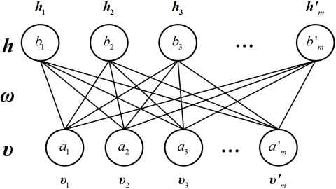
The RBM is a type of Markov random field and also an energy-based model. As shown in Figure 1, the RBM is a typical undirected graph, where the visible layer v is connected to the hidden layer h via undirected weighted connections.
Figure 1. The structure of the RBM
However, there is no connection between the nodes within the visible layer v or the hidden layer h. The high-order correlation can be reflected in the output of the hidden layer. The RBM can define a probability distribution model p(v,h;θ) based on an energy function E(v,h;θ). For a binary RBM, we have:
$\begin{align} & -\log p(v,h)\infty E(v,h;\theta ) \\ & =-\sum\limits_{i=1}^{\left| V \right|}{\sum\limits_{j=1}^{\left| H \right|}{{{w}_{ij}}{{v}_{i}}{{h}_{j}}}}-\sum\limits_{i=1}^{\left| V \right|}{{{b}_{i}}{{v}_{i}}}-\sum\limits_{j=1}^{\left| H \right|}{{{a}_{j}}{{h}_{j}}} \\ \end{align}$ (1)
where, θ=(w,a,b) is the set of parameters; wij is the connection weight between visible layer node I and hidden layer node j; aj and bi are the biases of the visible layer and the hidden layer, respectively; |V| and |H| are the number of visible layer nodes and hidden layer nodes, respectively. If v and h remain unchanged, the conditional probability distribution can be computed easily by:
$p({{h}_{j}}\left| v \right.;\theta )=sigm(\sum\limits_{i=1}^{\left| V \right|}{{{w}_{ij}}{{v}_{i}}}+{{a}_{j}})$ (2)
$p({{v}_{i}}\left| h \right.;\theta )=sigm(\sum\limits_{j=1}^{\left| H \right|}{{{w}_{ij}}{{h}_{j}}}+{{b}_{i}})$ (3)
where, sigm(x)=(1/(1+e-x)) is a sigmoid function. The parameter set θ=(w,a,b) can be learned through Contrastive divergence (CD-k) algorithm [23].
2.2 DBN
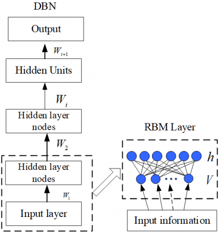
In the traditional DBN, the bottom layer is a stack of RBMs, while the top layer uses the BP algorithm for global finetuning (i.e. computing the error of each layer and adjusting the weight and bias of each layer). The network is a supervised learning with data labels as supervisory signals. The structure of the DBN is illustrated in Figure 2 below.
Figure 2. The structure of the DBN
The DBN is trained by a series of RBMs. The core idea of the training can be explained as follows: The parameter set θ=(w,a,b) obtained through RBM training can be used to define p(v|h,θ) and prior distribution p(h|θ). Hence, the probability of generating a visible layer node can be written as:
$p(v)=\sum\limits_{h}{p(\left. h \right|\theta )p(\left. v \right|h,\theta )}$ (4)
Once the parameter set θ has been learned from an RBM, the p(v|h,θ) will remain constant. In addition, p(h|θ) can be replaced by a continuous RBM, i.e. the hidden layer of the previous RBM can be treated as visible input. Therefore, the DBN can serve as an unsupervised feature learning method, in the absence of data labels.
2.3 ESN
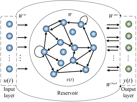
The ESN is a special form of recurrent neural network. As shown in Figure 3, an ESN is generally composed of an input layer, a dynamic reservoir and an output layer.
Figure 3. The structure of the ESN
The state update of the reservoir and the network output can be respectively defined as:
$u(n)=f({{W}_{res}}u(n-1)+{{W}_{in}}x(n))$ (5)
$y(n)={{f}_{out}}({{W}_{out}}u(n))$ (6)
where, $x(n)\in {{C}^{D\times 1}}$ and $y(n)\in {{C}^{K\times 1}}$are the input and output signals of the ESN, respectively; $u(n)\in {{C}^{N\times 1}}$ is the internal state of the reservoir at t=n; Wres is the internal weight matrix of the reservoir. Let N, D and K be a reservoir node, an input layer node and an output layer node, respectively. Then, the weights of linear input and linear output can be described as ${{W}_{in}}\in {{C}^{N\times D}}$ and ${{W}_{out}}\in {{C}^{K\times N}}$, respectively. The tanh function is generally adopted as the activation function f(•) of the reservoir, and fout as the readout function of the output layer. The fout can be a simple function selected manually (e.g. fout(•)=1) or a complex function.
In the ESN, the weight matrix Win of the input layer and the weight matrix Wres of the reservoir require no training. Both of them are randomly generated and constant. The only parameter to be trained is the weight matrix Wout of the output layer, which is generally trained by pseudo-inversion of known sequence. The ESN boasts a very useful function called the short-term memory, because the numerous sparsely connected neurons in the reservoir can record the state of the network before operation. As a result, this network is suitable for predicting factors that are highly correlated with the historical data, namely, tourist flow, traffic flow and shipping traffic.
To set up our tourist flow prediction model, the first step is to improve the traditional binary DBN. The tourist flow data were constructed based on real value units with Gaussian noise. Then, the conditional probability distribution and energy function can be written as:
$\begin{align} & -\log p(v,h)\infty E(v,h;\theta ) \\ & =\sum\limits_{i=1}^{\left| V \right|}{\frac{{{({{v}_{i}}-{{b}_{i}})}^{2}}}{2\sigma _{i}^{2}}}-\sum\limits_{j=1}^{\left| H \right|}{{{a}_{j}}{{h}_{j}}}-\sum\limits_{i=1}^{\left| V \right|}{\sum\limits_{j=1}^{\left| H \right|}{\frac{{{v}_{i}}}{{{\sigma }_{i}}}}}{{h}_{j}}{{w}_{ij}} \\ \end{align}$ (7)
$p({{h}_{j}}\left| v \right.;\theta )=sigm(\sum\limits_{i=1}^{\left| V \right|}{{{w}_{ij}}{{v}_{i}}}+{{a}_{j}})$ (8)
$p({{v}_{i}}\left| h \right.;\theta )=N({{b}_{i}}+{{\sigma }_{i}}\sum\limits_{j=1}^{\left| H \right|}{{{h}_{j}}{{w}_{ij}}},\sigma _{i}^{2})$ (9)
where, σ is the standard deviation vector; $N(\mu ,\sigma _{i}^{2})$ is the Gaussian distribution with the mean of σ and the variance of μ. The learning of wij is realized through CD-k. The weight update formula can be expressed as:
$\Delta {{w}_{ij}}=\eta ({{\left\langle {{v}_{i}},{{h}_{j}} \right\rangle }_{data}}-{{\left\langle {{v}_{i}},{{h}_{j}} \right\rangle }_{recon}})$ (10)
where, η is the learning rate.
Before inputting the tourist flow data, the sparse model must be regularized first. The activation function with regularization penalty can be described as:
$\lambda \sum\limits_{j=1}^{\left| H \right|}{{{(\rho -\frac{1}{m}(\sum\limits_{k=1}^{m}{E\left[ {{h}_{j}}\left| {{v}^{k}} \right. \right]}))}^{2}}}$ (11)
where, vk is a sample in the training set; ρ is sparsity.
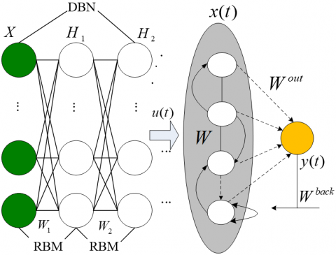
Figure 4. ESN-DBN tourist flow prediction model
As shown in Figure 4, the DBN was improved based on the ESN. Specifically, the highest-level data features eventually extracted by the RBMs in the DBN were expressed as ${{H}^{p}}=\left\{ h_{1}^{p},h_{2}^{p},\ldots ,h_{m}^{p} \right\}$, where p is the top layer and m is the number of top layer features. In the architecture of our model, the most representative feature Hp was taken as the input vector for prediction (the ESN layer of the top layer). The operations of the proposed ESN-DBN model can be summed up as follows: the DBN learns representative and robust features from the inputs through multi-layer nonlinear feature transformation, and uses them to describe the complex mappings of the inputs and features in the tourism system; then, the prediction results are generated in the ESN regression layer based on the DBN features.
During the supervised ESN training at the top level, the weights between reserve state and output layer state can be updated by:
$\begin{align} & x(t+1)=f({{W}^{in}}u(t+1)+Wx(t)+{{W}^{back}}y(t)) \\ & y(t+1)={{W}^{out}}x(t+1) \\ \end{align}$ (12)
where, x(t) and y(t) are the input and output signals of the reservoir, respectively; W is the weight matrix of internal connections of the reservoir; Win and Wout are the weight matrices of input layer and output layer, respectively; Wback is the feedback matrix initialized randomly from the mean distribution. The tanh function was adopted as the activation function f(•) of neurons. The local weight adjustment of the ESN is explained in Table 1.
Table 1. Local weight adjustment of the ESN
|
Algorithm 1: Local weight adjustment of the ESN |
|
Inputs: u(t), x(t), y(t), λ (the spectral radius), Win, W, Wout h1 (the state of the final DBN output). Output: Wout (the weight matrix of the output layer) 1: Network initialization 2: Random definition of Win, W and Wout 3: $\lambda \in \left( 0,1 \right)$ 4: x(0)=0 5: Dynamic sampling for network training 6: u(t)←h1 7: for t=0 to T do 8: Updating the reservoir state 9: Setting up the reservoir state matrix X 10: Setting up the output layer matrix Y 11: Computing the output layer weight matrix |
The ESN-DBN algorithm can be implemented in the following steps:
Step 1. Initialize network parameters (Wi,bi) (1≤i≤r+1) as a close-to-zero random number.
Step 2. Train the first RBM by CD-k and denote its visible layer as v and hidden layer as h1.
Step 3. For(1≤i≤r-1), take hi-1 and hi as the visible layer and the hidden layer of the i-th RBM, respectively; train the RBM layer by layer by CD-k.
Step 4. For i=r, set up a RBM classifier with hr-1 and y as the visible layer and hr as the hidden layer, and train the RBM classifier by CD-k.
Step 5. Take the biases between the trained RBMs as the initial weight and bias of the ESN, and finetune the local weight and bias of each layer based on the ESN.
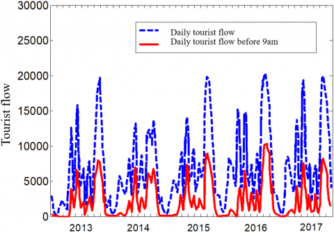
The predictive performance of the ESN-DBN was verified through experiments, and compared with that of the BPNN and the classical ARIMA. For our experiments, the tourist flow dataset of seven yearly holidays (2013-2017) was collected from a tourist center. As shown in Figure 5, the dataset covers both the daily tourist flow on holidays, and the daily tourist flow before 9am on holidays. The data in 2013-2016 were taken as the training set, and the data in 2017 was adopted to verify the prediction results.
Figure 5. Holiday tourist flow dataset 2013-2017
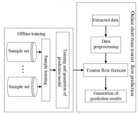
The model prediction was divided into two parts, aiming to enhance the real-time performance of the prediction and reduce the time lag of online data training. First, the preliminary prediction model was obtained through offline training based on historical data. Next, the prediction process was further optimized. Offline training can greatly shorten the computing time of the prediction model, because it does not occupy the time for online data prediction of the ESN-DBN. Figure 5 presents the structure of the ESN-DBN prediction model for tourist flow.
Figure 6. The structure of the ESN-DBN prediction model for tourist flow
The parameters of our ESN-DBN were calibrated empirically and adjusted through trial-and-error. Each RBM has three hidden layers, each of which has 30 nodes. The learning rate and number of iterations are 0.1 and 450, respectively. The sigmoid function was adopted as the activation function. In the ESN, the initial number of nodes was set to 60. The experiments were conducted on Matlab2018b in Windows 10, using the same hardware (Intel Core i7-6850K-3.60GHz; RAM 16G).
The ESN-DBN was compared with the BPNN and the ARIMA in terms of accuracy and computing time. The prediction accuracy was measured by three indices, namely, mean absolute error (MAE), root-mean-square error (RMSE) and mean absolute percentage error (MAPE):
$MAE=\frac{1}{n}\sum\limits_{i=1}^{n}{\left| {{y}_{i}}(i)-{{{{y}'}}_{i}}(i) \right|}$ (13)
$RMSE=\sqrt{\frac{1}{n}\sum\limits_{i=1}^{n}{{{({{y}_{i}}(i)-{{{{y}'}}_{i}}(i))}^{2}}}}$ (14)
$MAPE(y,{y}')=\frac{1}{n}\sum\limits_{i=1}^{n}{\frac{\left| {{y}_{i}}-{{{{y}'}}_{i}} \right|}{{{y}_{i}}}}$ (15)
where, yi is the actual value; $\mathcal { y } _ { i } ^ { \prime }$ is the predicted value.
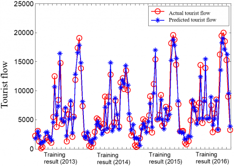
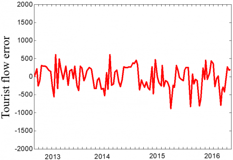
The ESN-DBN was trained by the data in 2013-2016. The actual tourist flow in each year was compared with that predicted by the trained model (Figures 7 and 8). It can be seen that the curve of predicted tourist flow basically has the same trend with that of actual tourist flow, and the prediction error was controlled within 6%.
Figure 7. Training results
Figure 8. Prediction error
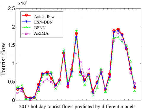
Furthermore, the ESN-DBN was applied to predict the holiday tourist flow in 2017, and compared with the prediction results of the BPNN and the ARIMA. The comparison is illustrated in Figure 9 below.
Figure 9. The 2017 holiday tourist flows predicted by different models
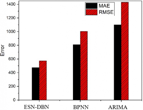
The MAEs and RMSEs of the three models in tourist flow prediction are displayed in Figure 10. The three models were also compared by the MAPE and computing time (Table 2).
Figure 10. MAE and RMSE of the three models
Table 2. Comparison of the three models in prediction accuracy and computing time
|
Model |
Accuracy and computing time |
|||
|
MAPE |
MAE |
RMSE |
Mean computing time/s |
|
|
ARIMA |
23.87% |
1,100 |
1,430 |
12 |
|
BPNN |
19.07% |
810 |
1,004 |
30 |
|
ESN-DBN |
11.25% |
475 |
573 |
24 |
It can be seen that the MAE and RMSE of the proposed ESN-DBN were 475 and 573, respectively, those of the ARIMA were 1,100 and 1,430, respectively, and those of the BPNN were 810 and 1,004, respectively. Hence, the ARIMA had the poorest predictive performance, due to the high nonlinearity of tourist flow; the ESN-DBN achieved better prediction accuracy than the BPNN, which has a shallow structure. The MAPEs of the BPNN, ARIMA and ESN-DBN were respectively 19.07%, 23.87% and 11.25%, indicating that our model boasts the most accurate prediction of tourist flow.
This paper introduces the ESN to improve the DBN for tourist flow prediction. In the proposed ESN-DBN, the bottom layer is a stack of RBMs that extract features from the input historical data, and the top layer is an ESN-based DL prediction model for tourist flow. The bottom layer adopts the structure of a typical DBN and could realize unsupervised feature learning in an effective manner. The ESN is effectively integrated with the DBN to perform supervised learning in the decision-making layer. In this way, the weights and biases of the entire network are adjusted, such that the network can effectively map the complex relationship in the tourism network. Several experiments were conducted on actual dataset of holiday tourist flow. The results prove that the ESN-DBN enhances the prediction accuracy of tourist flow, because it can carry out effective feature learning with very limited prior knowledge. In addition, it is learned that the ESN-DBN outperformed the BPNN and ARIMA in prediction performance, realizing the lowest MAE and RMSE. What is more, the ESN-DBN also achieved the lower MAPE (11.25%) than the two contrastive models. The computing time of the ESN-DBN fell between that of the ARIMA and that of the BPNN, and basically satisfies the requirement on computing speed. With these advantages, the ESN-DBN can be applied to the tourist system very easily. The future research will optimize the ESN-DBN to further reduce its computing time, and will promote the model to tourist flow prediction in even shorter periods.
[1] Li, X., Pan, B., Law, R., Huang, X.K. (2017). Forecasting tourism demand with composite search index. Tourism Management, 59: 57-66. https://doi.org/10.1016/j.tourman.2016.07.005
[2] Shen, W., Liu-Lastres, B., Pennington-Gray, L., Hu, X.H., Liu, J.Y. (2018). Industry convergence in rural tourism development: A China-featured term or a new initiative? Current Issues in Tourism, 22(20): 2453-2457. https://doi.org/10.1080/13683500.2018.1532396
[3] Ruan, W.Q., Li, Y.Q., Zhang, S.N., Liu, C.H. (2019). Evaluation and drive mechanism of tourism ecological security based on the DPSIR-DEA model. Tourism Management, 75: 609-625. https://doi.org/10.1016/j.tourman.2019.06.021
[4] Yang, X., Pan, B., Evans, J.A., Lv, B. (2015). Forecasting Chinese tourist volume with search engine data. Tourism Management, 46: 386-397. https://doi.org/10.1016/j.tourman.2014.07.019
[5] Burger, C., Dohnal, M., Kathrada, M., Law, R. (2001). A practitioners guide to time-series methods for tourism demand forecasting-a case study of Durban, South Africa. Tourism Management, 22(4): 403-409. http://dx.doi.org/10.1016/S0261-5177(00)00068-6
[6] Kim, J.H., Ngo, M.T. (2001). Modelling and forecasting monthly airline passenger flows among three major Australian cities. Tourism Economics, 7(4): 397-412. http://dx.doi.org/10.5367/000000001101297946
[7] Chu, F.L. (2009). Forecasting tourism demand with ARMA-based methods. Tourism Management, 30(5): 740-751. http://dx.doi.org/10.1016/j.tourman.2008.10.016
[8] Gustavsson, P., Nordström, J. (2001). The impact of seasonal unit roots and vector ARMA modelling on forecasting monthly tourism flows. Tourism Economics, 7(2): 117-133. http://dx.doi.org/10.5367/000000001101297766
[9] Lim, C., McAleer, M. (2002). Time series forecasts of international travel demand for Australia. Tourism Management, 23(4): 389-396. http://dx.doi.org/10.1016/S0261-5177(01)00098-X
[10] Goh, C., Law, R. (2002). Modeling and forecasting tourism demand for arrivals with stochastic nonstationary seasonality and intervention. Tourism Management, 23(5): 499-510. http://dx.doi.org/10.1016/S0261-5177(02)00009-2
[11] Lakshmipathi, A.N., Battula, B.P. (2018). Deep convolutional neural networks for product recommendation. Ingénierie des Systèmes d’Information, 23(6): 161-172. https://doi.org/10.3166/ISI.23.6.161-172
[12] Cetinic, E., Lipic, T., Grgic, S. (2018). Fine-tuning convolutional neural networks for fine art classification. Expert Systems with Applications, 114: 107-118. https://doi.org/10.1016/j.eswa.2018.07.026
[13] Wang, X., Wang, L., Li, S., Wang, J. (2018). An event-driven plan recognition algorithm based on intuitionistic fuzzy theory. Journal of Supercomputing, 74(12): 6923-6938. https://doi.org/10.1007/s11227-018-2650-9
[14] Pai, P.F., Hong, W.C. (2005). An improved neural network model in forecasting arrivals. Annals of Tourism Research, 32(4): 1138-1141. http://dx.doi.org/10.1016/j.annals.2005.01.002
[15] Claveria, O., Monte, E., Torra, S. (2015). Tourism demand forecasting with neural network models: Different ways of treating information. International Journal of Tourism Research, 17(5): 492-500. http://dx.doi.org/10.1002/jtr.2016
[16] Cao, G., Wu, L. (2016). Support vector regression with fruit fly optimization algorithm for seasonal electricity consumption forecasting. Energy, 115: 734-745. http://dx.doi.org/10.1016/j.energy.2016.09.065
[17] Mariani, M., Baggio, R., Fuchs, M., Höepken, W. (2018). Business intelligence and big data in hospitality and tourism: A systematic literature review. International Journal of Contemporary Hospitality Management, 30(12): 3514-3554. http://dx.doi.org/10.1108/IJCHM-07-2017-0461
[18] Yao, Y., Cao, Y., Ding, X., Zhai, J., Liu, J.X., Luo, Y.L., Ma, S., Zou, K.L. (2018). A paired neural network model for tourist arrival forecasting. Expert Systems with Applications, 114: 588-614. https://doi.org/10.1016/j.eswa.2018.08.025
[19] Sun, J., Chang, T. (2016). Prediction of rural residents' tourism demand based on back propagation neural network. International Journal of Applied Decision Sciences, 9(3): 320-331. http://dx.doi.org/10.1504/IJADS.2016.081095
[20] Hong, W.C., Dong, Y., Chen, L.Y., Wei, S.Y. (2011). SVR with hybrid chaotic genetic algorithms for tourism demand forecasting. Applied Soft Computing, 11(2): 1881-1890. https://doi.org/10.1016/j.asoc.2010.06.003
[21] Chen, R., Liang, C.Y., Hong, W.C., Gu, D.X. (2015). Forecasting holiday daily tourist flow based on seasonal support vector regression with adaptive genetic algorithm. Applied Soft Computing, 26: 435-443. https://doi.org/10.1016/j.asoc.2014.10.022
[22] Huang, W., Song, G., Hong, H., Xie, K.Q. (2014). Deep architecture for traffic flow prediction: deep belief networks with multitask learning. IEEE Transactions on Intelligent Transportation Systems, 15(5): 2191-2201. http://dx.doi.org/10.1109/TITS.2014.2311123
[23] Hinton, G.E., Osindero, S., Teh, Y.W. (2006). A fast learning algorithm for deep belief nets. Neural Computation, 18(7): 1527-1554. http://dx.doi.org/10.1162/neco.2006.18.7.1527