Yuhe Wang | Peili Qiao* | Guanglu Sun | Kai Fan | Xin Zeng
OPEN ACCESS
During data classification, the classifier often performs poorly facing imbalanced dataset. To solve the problem, this paper develops a classification method, denoted as the IRWM, for imbalanced dataset based on the random walk model (RWM). Firstly, a positive example and a negative example were set up according to the imbalance of the training data. Then, the training data were mapped separately into the random walk graph (RWG) for the positive example and that for the negative example. Once inputted, each data was walked separately in the two RWGs, yielding two probabilities. After that, the two probabilities of the unclassified data were compared with the preset comparison coefficient to determine the final class of the data. The proposed method was contrasted with the support vector machine (SVM) algorithm through experiments. The results show that our method can effectively classify data in imbalanced dataset.
imbalanced dataset, random walk model (RWM), data classification, support vector machine (SVM), random walk probability
The classification of data, especially the complex data, is both a hot spot and difficult point in the current research. The research difficulty partly comes from the imbalance of data distribution in the real world, such as rare disease monitoring data, machine fault data, etc. [1]. In an imbalanced dataset, there are far more samples in one class than those in another class. More and more scholars have attempted to accurately classify data in such a dataset. The existing classification methods for imbalanced data fall into three categories: data-side method, the classifier-side method, and the hybrid method. The data-side method carries out classification after reducing the data complexity through preprocessing; the classifier-side method designs special classifier that suits the data complexity; the hybrid method combines the previous two methods.
Many scholars at home and abroad have explored the classification of imbalanced data. For example, Chen et al. [2] puts forward a classification method for imbalanced data based on the borderline synthetic minority over-sampling technique (BSMOTE), which enhances the classification accuracy of a few samples by reversing the imbalance ratio and integrating multiple classification methods. Considering the support vector sparsity of traditional classification methods, Zhang et al. [3] speeds up the classification through k-means clustering of support vectors and extraction of new support vectors from the cluster centers. Han et al. [4] designs an integrated classifier coupling the rotation forest and the extreme learning machine, aiming to solve the overfitting in the classification process and improve the classification accuracy. On the classification of imbalanced dataset, Gónzalez et al. [5] proposed a method based on the distance to the closest energy to overcome the data shortage of imbalanced dataset. Sankalp Jain et al. [6] applied the random forest model to develop a prediction model for the imbalanced dataset on silicon element. Bamakan [7] improved the k-support vector classification regression (K-SVCR) model, and adopted it to solve the data imbalance in network intrusion detection. To sum up, the existing classification methods for imbalanced data need to be further improved to accurately classify the complex and changing data in the real world.
This paper probes deep into the classification of imbalanced data, and proposes an imbalanced dataset classification method based on random walk model (IRWM). Specifically, the plotting of the random walk graph (RWG) for the imbalanced dataset was taken as the training process. Considering the data imbalance, the training dataset was mapped into two RWGs, one for positive example and the other for negative example, and used to execute the walks. Two stable probability distributions were obtained through the walks. Next, the two probabilities were compared according to the comparison coefficient to determine the class of the unclassified data. In this way, the data flooding caused by the imbalance was overcame, making it possible to realize accurate classification. In addition, the classification results can be controlled by adjusting the probability comparison coefficient according to the specific imbalance ratio, as the probability of unclassified data falling into each class can be obtained by walking.
The imbalanced dataset is defined as a dataset containing far fewer samples in one class than those in other classes, and this class is the only one worthy of attention. Data imbalance is commonplace in real life. For instance, the failure data are outnumbered by normal data in the detection of system failures; there are far more normal cells than abnormal cells in disease diagnosis; abnormal samples are way fewer than normal samples in network intrusion detection, spam mail classification, crank call identification and automatic text classification. In this paper, the imbalanced dataset is divided into two parts, namely, a positive example dataset of small samples and a negative example dataset of large samples. Note that the number of small samples are much greater than that of large samples.
The support vector machine (SVM), an effective way to retrieve information, recognize images and classify texts, performs poorly facing data imbalance. The poor performance is attributable to two inherent constraints on imbalanced data: information deficiency and information bias. The former refers to the number of samples, i.e. the amount of information in the positive example, while the latter stands for the ratio of the number of samples between the positive example and the negative example, that is, the imbalance ratio of the dataset. Under the two inherent constraints, the support vectors of the positive example are outnumbered by those of the negative example, such that the negative example is favored by the classification decision function [8].
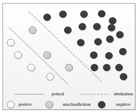
Figure 1. The effects of information deficiency on classification
Figure 2. The effects of information bias on classification
Figure 1 explains the effects of information deficiency on classification. Since the imbalanced dataset contains too few samples of the positive example, there is a lack of information on the positive example during the classification. During the training, some samples of the positive example will be misclassified into the negative example, due to the information deficiency. This will dampen the accuracy of the classification results.
Figure 2 illustrates the effects of information bias on classification. The continuous growth in imbalance of the dataset will exacerbate the data flooding effect, that is, the shift of classification results to the positive example. As a result, some samples of the positive example will be misclassified into the negative example and the inverse is true. This will also reduce the classification accuracy.
Considering the inherent constraints and classification problems of imbalanced dataset, this paper puts forward a classification strategy by improving the random walk model (RWM), which can avoid the hyperplane offset of the trained dataset.
Based on the RWM, the RIWM algorithm fully considers the two inherent constraints of imbalanced dataset, and lays the basis for a classification model suitable for imbalanced data, offering an effective strategy for classifying imbalanced dataset.
3.1 Random walk model
Random walk means the past performance of the target cannot be used to predict its future development or trend [9]. The RWM has been widely adopted in computer fields like data mining and image processing. This model often solves classification problems (e.g. multi-label classification) through a time stochastic process. Google’s PageRank algorithm is an example of the RWM [10].
The first step of RWM solution is to establish a connected RWG that can be mapped onto the object. The connected RWG could be directed or undirected, depending on the actual conditions. The second step is to set up a weight matrix. The final step is to walk on the RWG using the random walk algorithm, i.e. transverse the entire graph from one or a series of fixed points. The walking process is detailed as follows: From any fixed point, the traveler will walk to an adjacent fixed point at the probability of 1-α, or jump to any other fixed point at the probability of $1-\alpha$. Here, $\alpha$ is called the jump probability. A probability distribution can be obtained after each walk. Each state either remains the same or mutates into another state according to the probability distribution. The jump between states is independent of the previous state and only depends on the current state. In other words, the entire process is memoryless. The obtained probability distribution is the probability set that each vertex in the whole graph is visited, and adopted as the input of the next walk. The walking process is iterated until the probability distribution tends to converge. After convergence, a stable probability distribution can be obtained. The final probability can be regarded as the walk probability of the data in the RWG [11].
3.2 IRWM algorithm flow
Definition 1: Let X be the set d-dimensional data in the real number field R:
$X=R^{d}$ (1)
Definition 2: Let Y be the set of all class labels in the classification process:
$Y=\left\{y_{\text {Positive }}, y_{\text {Negative }}\right\}$ (2)
Definition 3: Let D be a set of training data containing m samples:
$D=\left\{\left(x_{i}, y_{i}\right) | 1 \leq i \leq m, y_{i} \in Y\right\}$ (3)
where, xi is a training data in X; yi is the true class of xi.
3.2.1 Setting up the RWGs
To begin with, the dataset should be divided into a test dataset and a training dataset D, and map the latter into a d-dimensional RWG. Considering the binary division of imbalanced dataset, this paper maps the training dataset into two RWGs, namely, the RWG for positive example (PRWG) and the RWG for negative example (NRWG). In the RWGs, the connection between the fixed points mirrors the relationship between the various training data [12].
Definition 4: Let v be the fixed points in the RGWs corresponding to the data x (x∈X) in the training dataset D. If xi and xj belong to the same class, then link up the corresponding fixed points vi and vj in the RGWs. The PRWG and NRWG can be described as:
$G=(V, E)$ (4)
$V=\left\{v_{i} | x_{i} \in X, 1 \leq i \leq m\right\}$ (5)
$E=\left\{\left(v_{i}, v_{j}\right) | v_{i}, v_{j} \in V, i \neq j\right\}$ (6)
3.2.2 Calculating the weight matrix
Definition 5: Let the Euclidean distance dis(vi,vj) be the weight coefficient of the edge between each pair of vertices, i.e. the distance of each sample in the d- dimensional space:
$\operatorname{dis}\left(v_{i}, v_{j}\right)=\sqrt{\sum_{k=1}^{d}\left(x_{i k}-x_{j k}\right)^{2}}$ (7)
Taking dis(vi,vj) as the weight coefficient, compute the weight W in the RWGs according to individual difference between vertices as follows:
$W_{i j}=\left\{\begin{array}{ll}{0,} & {v_{i}=v_{j}} \\ {\infty,} & {v_{i} \neq v_{j},\left(v_{i}, v_{j}\right) \notin E} \\ {\operatorname{dis}\left(v_{i}, v_{j}\right)} & {v_{i} \neq v_{j},\left(v_{i}, v_{j}\right) \in E}\end{array}\right.$ (8)
In the d-dimensional space, samples vi and vj can be respectively expressed as:
$v_{i}=\left(x_{i 1}, x_{i 2}, \ldots, x_{i d}\right)$ (9)
$v_{i}=\left(x_{i 1}, x_{i 2}, \ldots, x_{i d}\right)$ (10)
3.2.3 Walking preparations of unclassified data
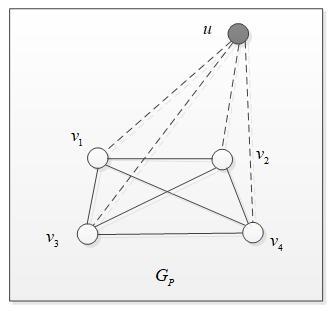
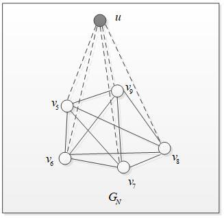
The unclassified data was entered into the RWGs for walking and classification according to the RWM. Let u be the fixed point corresponding to data x, and Gp be the graph obtained by linking up u with each point in the PRWG. As shown in Figure 3, v1, v2, v3 and v4 are the vertices corresponding to the samples in the positive example. Similarly, the graph GN can be obtained by linking up u with each point in the NRWG. As shown in Figure 4, v5, v6, v7, v8 and v9 are the vertices corresponding to the samples in the negative sample. The walk will start from u on both Gp and GN.
Figure 3. The PRWG
Figure 4. The NRWG
The normalized form of Gp and GN can be expressed as:
$G^{\prime}=\left(V^{\prime}, E^{\prime}\right)$ (11)
$V^{\prime}=V \cup\{u\}$ (12)
$E^{\prime}=E \cup\left\{\left(u, v_{i}\right) | 1 \leq i \leq m\right\}$ (13)
Before performing random walks on unclassified data with u as the starting point, the following three items should be calculated:
(1) The m-dimensional initial vector λ0
First, the value of $\lambda_{0}^{\prime}$ can be calculated by:
$\lambda_{0}^{\prime}(i)=\left\{\begin{array}{ll}{\operatorname{dis}\left(u, v_{i}\right),} & {\left(u, v_{i}\right) \in E^{\prime}} \\ {0,} & {\text { otherwise }}\end{array}\right.$ (14)
Then, the initial vector λ0 can be obtained by normalizing $\lambda_{0}^{\prime}$:
$\lambda_{0}=\frac{\lambda_{0}^{\prime}-\operatorname{avg}\left\{\lambda_{0}^{\prime}\right\}}{\operatorname{std}\left\{\lambda_{0}^{\prime}\right\}}$ (15)
(2) The adjacency matrix P
For any vertex v, the probability that the unclassified data walks to an adjacent vertex of v is negatively correlated with the distance between v and that vertex. The matrix Mij can be obtained by:
$M_{i j}=\frac{W_{i j}}{\max _{1 \leq k \leq m}\left\{W_{i j} | W_{k j} \neq \infty\right\}}$ (16)
The matrix Mij can be normalized as:
$M_{i j}^{\prime}=\frac{M_{i j}-\operatorname{avg}_{i}\left\{M_{i j}\right\}}{\operatorname{std}_{i}\left\{M_{i j}\right\}}$ (17)
From formulas (16) and (17), we can derive matrix Pij:
$P_{i j}=\frac{M_{j}^{\prime}}{\sum_{i} M_{i j}^{\prime}}$ (18)
(3) The distribution of the jump probability d
The previous studies have shown that the classification results are desirable if α falls in 0.40~0.90 [12]. In this paper, the value of α is set to a medium value: 0.65. Assuming that the jump probability from a certain point to any other fixed point is constant, then the distribution of the jump probability d can be expressed as:
$d=\left\{\frac{1}{m}, \frac{1}{m}, \frac{1}{m}, \ldots, \frac{1}{m}\right\}$ (19)
3.2.4 Random walking of unclassified data
The unclassified data were subjected to random walking according to the above steps. After each walk, a probability distribution vector λ can be computed and outputted based on the RWGs GP and GN:
$\lambda=(1-\alpha) \cdot P^{T} \cdot \lambda_{0}+\alpha \cdot d$ (20)
Taking λ as λ0 in formula (15), a stable probability distribution vector z can be obtained through iterative convergence:
$z=(1-\alpha) \cdot P^{T} \cdot z+\alpha \cdot d$ (21)
where, z is the conditional probability to transverse each RWG, i.e. GP or GN. Let z(i) be the probability to walk from point u to point vi. Then, $z=(1-\alpha) \cdot P^{T} \cdot z+\alpha \cdot d$, the mean value of elements in z, can be calculated by:
$\overline{P}=\operatorname{avg}(\{z(i) | 1 \leq i \leq m\})$ (22)
According to the conditional probability model, Px, the probability that the unclassified data x belongs to the current class can be expressed as:
$P_{x}=\left(\overline{P}_{P}+\overline{P}_{N}\right) \cdot P_{r}$ (23)
where, Pr is the prior probability that the unclassified data x is connected to a point in GP or GN; $\overline{P}_{P}$ and $\overline{P}_{N}$ are the mean conditional probabilities obtained through the walk on the PRWG and the NRWG, respectively. Then, s, the mean similarity of x to all samples in that class can be described as:
$s=\operatorname{avg}\left\{A \operatorname{Cos}\left(x, v_{i}\right)\right\}$ (24)
Finally, the prior probability Pr can be obtained through the normalization by formulas (11)-(13).
3.2.5 Classification of unclassified data
After unclassified data completed the random walks on the RWGs, two probabilities PP and PN were obtained from the PRWG and the NRWG, respectively. Under the effect of information bias, the datasets of different imbalance ratios cannot be classified by the same standard. Hence, an adjustable comparison coefficient β (0<β≤1) was designed to ensure the classification accuracy. Different β values were tested to disclose how the coefficient affects the accuracy of data classification.
4.1 Datasets
The classification effect of the proposed algorithm was verified through experiments on four public datasets from the UCI Machine Learning Repository. The datasets were preprocessed into the basic datasets of our experiments (Table 1).
Table 1. Experimental datasets
|
Name |
Number of samples |
Imbalance ratio |
Number of positive samples |
Dataset condition |
|
Cardiotocography |
2126 |
138.2:1 |
29 |
High imbalance ratio and low information volume |
|
Census Income |
48842 |
206.8:1 |
235 |
High imbalance ratio and high information volume |
|
University |
285 |
7.9:1 |
32 |
Low imbalance ratio and low information volume |
|
Advertise-ments |
3279 |
5.7:1 |
487 |
Low imbalance ratio and high information volume |
4.2 Evaluation indices
In view of the dataset imbalance, the confidence of the classification algorithm was measured by the receiver operating characteristic (ROC) curve and the area under the curve (AUC). There are four possible outcomes of imbalanced dataset classification: the true positive (TP), the false positive (FP), the true negative (TN) and the false negative (FN). The TP means a positive example is correctly predicted as a positive one; the FP means a negative example is mistaken as a positive one; the TN means a negative example is correctly predicted as a negative one; the FN means a positive example is mistaken as a negative one.
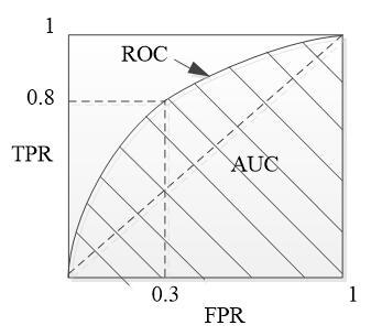
As shown in Figure 5, the ROC curve is a graphical representation of the compromise between the true positive rate (TPR) and the false positive rate (FPR) of the classification results:
$T P R=\frac{T P}{T P+F N}=\frac{T P}{P}$ (25)
$F P R=\frac{F P}{F P+T N}=\frac{F P}{P}$ (26)
The closer the ROC curve gets to the upper left corner, the better the performance of the classifier. Compared with the ROC curve, the AUC can offer a clear, intuitive display of the mean performance of the classifier. In Figure 5, the AUC stands for the area under the ROC curve. Here, the AUC value is calculated by mathematical integration. The closer the AUC value gets to 1, the better the performance of the classifier [14].
Figure 5. The ROC curve and the AUC
4.3 Experimental process and results analysis
Firstly, the training dataset was classified by random sampling. Half of the sample data was randomly selected as the training dataset, and the other half was taken as the test dataset. The two datasets have the same ratio of the number of samples between the positive example and the negative example. Next, the IRWM and the SVM were applied to the four experimental datasets. Note that the comparison coefficient of the IRWM was set to β=1, and the penalty factor of the SVM was set to C=1. The ROC values obtained by the two algorithms on the four datasets are compared in Figures 6-9 below. Finally, the effects of β in the IRWM on the classification accuracy were tested.
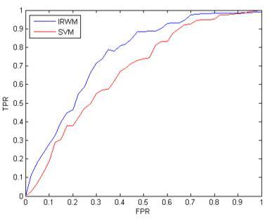
Figure 6. Experimental results on cardiotocography dataset
Figure 7. Experimental results on census income dataset
Figure 8. Experimental results on university dataset
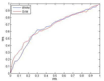
Figure 9. Experimental results on advertisement dataset
As shown in Figures 6-9, the IRWM outputted better classification results than the SVM under three conditions, namely, high imbalance ratio and low information volume, high imbalance ratio and high information volume, as well as low imbalance ratio and low information volume. Under low imbalance ratio and high information volume, our method still achieved comparable accuracy to that of the SVM.
To further compare the accuracies of the two methods, the AUCs obtained by the SVM and the IRWM on the four datasets were compared in details (Table 2).
Table 2. The AUCs of the two algorithms
|
Algorithms |
Cardiotoco-graphy |
Census Income |
University |
Advertise-ments |
|
SVM |
0.7539 |
0.6037 |
0.4698 |
0.7437 |
|
IRWM |
0.8137 |
0.8243 |
0.7574 |
0.7421 |
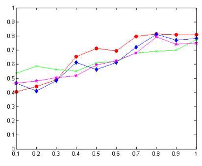
Figure 10 The effects of β value on classification accuracy
Figure 10 demonstrates a significant impact of the β value on the classification effect on imbalanced dataset. Overall, the classification is relatively accurate when the β value falls in 0.8-1.0.
This paper probes deep into the existing classification algorithms of imbalanced data, analyzes the effects of data imbalance on current classifiers, and designs a classification method specifically for imbalanced dataset. Based on the RWM, the proposed method firstly takes account of the information deficiency and information bias in the imbalanced data, plots the RWGs for the imbalanced data, and sets up the corresponding weights. Next, the unclassified data was classified through the walking on the PRWG and the NRWG. The comparative experiments confirm that the IRWM outperformed the SVM in the classification of imbalanced data. However, the comparison coefficient in our IRWM algorithm is yet to be improved, and the β value is quite sensitive to the dataset imbalance. The future research will improve our method from these two aspects, and further enhance the classification accuracy.
This work was supported in part by the Scientific Research Starting Foundation for Returned Overseas of Heilongjiang Province under Grants LC2018030.
[1] Li, Y., Liu, Z.D., Zhang, H.J. (2014). Review on ensemble algorithms for imbalanced data classification. Application Research of Computers, 31(5): 1287-1291. http://dx.chinadoi.cn/10.3969/j.issn.1001-3695.2014.05.002
[2] Chen, R., Zhang, L., Yang, J., Hu, R.G. (2014). Classification algorithm for imbalanced data sets based on combination of BSMOTE and inverse under sampling. Application Research of Computers, 31(11): 3299-3303. http://dx.chinadoi.cn/10.3969/j.issn.1001-3695.2014.11.023
[3] Zhang, Z.C., Wang, S.T., Deng, Z.H., Chung, F.L. (2011). Fast decision using SVM for incoming samples. Journal of Electronics & Information Technology, 33(9): 2181-2186. http://dx.chinadoi.cn/10.3724/SP.J.1146.2011.00107
[4] Han, M., Liu, B. (2013). An improved rotation forest classification algorithm. Journal of Electronics & Information Technology, 35(12): 2896-2900. http://dx.chinadoi.cn/10.3724/SP.J.1146.2012.01707
[5] Gónzalez, S., García, S., Lázaro, M., Figueiras-Vidal, A.R., Herrera, F. (2017). Class switching according to nearest enemy distance for learning from highly imbalanced data-sets. Pattern Recognition, 70: S0031320317301796. http://dx.doi.org/10.1016/j.patcog.2017.04.028
[6] Jain, S., Kotsampasakou, E., Ecker, G.F. (2018). Comparing the performance of meta-classifiers—A case study on selected imbalanced data sets relevant for prediction of liver toxicity. Journal of Computer-Aided Molecular Design, 32(5): 583-590. https://doi.org/10.1007/s10822-018-0116-z
[7] Bamakan, S.M.H., Wang, H., Shi, Y. (2017). Ramp loss k-support vector classification-regression; a robust and sparse multi-class approach to the intrusion detection problem. Knowledge-Based Systems, 126: 113-126. https://doi.org/10.1016/j.knosys.2017.03.012
[8] Tao, X.M., Hao, S.Y., Zhang, D.X., Xu, P. (2013). Kernel cluster-based ensemble SVM approaches for unbalanced data. Journal of Harbin Engineering University, 34(3): 381-388. http://dx.chinadoi.cn/10.3969/j.issn.1006-7043.201206069
[9] Ji, D.X., Sun, Y.Q. (2014). An improved random walk based community detection algorithm. International Journal of Multimedia and Ubiquitous Engineering, 9(5): 131-141. http://dx.doi.org/10.14257/ijmue.2014.9.5.12
[10] Tan, S.B., Wu, Q. (2011). A random walk algorithm for automatic construction of domain-oriented sentiment lexicon. Expert Systems with Applications, 38(10): 12094-12100.
[11] Zhen, W., Wang, Z.K. (2010). A multi-label classification algorithm based on random walk model. Chinese Journal of Computers, 33(8): 1418-1426. http://dx.chinadoi.cn/10.3724/SP.J.1016.2010.01418
[12] Yildirim, H., Krishnamoorthy, M.S. (2008). A random walk method for alleviating the sparsity problem in collaborative filtering. 2008 2nd ACM International Conference on Recommender Systems, RecSys, pp. 131-138. http://dx.doi.org/10.1145/1454008.1454031
[13] Feng, X.Y. (2016). Data sparseness of unbalanced data oriented research. Harbin University of Science and Technology, pp. 39-42.
[14] Ferri, C., Hernandez, O.J., Flach, P.A. (2011). A coherent interpretation of AUC as a measure of aggregated classification performance. Proceedings of the 28th International Conference on Machine Learning (ICML-11), pp. 657-664.