Amin Moslemi Petrudi*| Masoud Rahmani
© 2020 IIETA. This article is published by IIETA and is licensed under the CC BY 4.0 license (http://creativecommons.org/licenses/by/4.0/).
OPEN ACCESS
Composite laminates are widely used in civil engineering, aerospace, shipbuilding and the military industry because of their high strength and rigidity to their high weight ratio, good fatigue resistance and high energy absorption fineness. The mechanism of degradation in composites is very complex and one or more degradation modes may occur in the composites at the same time. In this paper, multi-layer composite degradation with stress concentration due to internal hole is investigated numerically and analytically. The miso-scale model is used to investigate the problem. Fortran and Ansys software have been used to analyze the problem. The usermat code is embedded in Fortran software and linked to Ansys software. The present paper solves the stress induced multilayers in the present study, and compares the results of this method with those of other researchers. Stress and damage contours have been reported. it is shown Change of the diameter of the central open-hole not only the effect on possible damage, damaging rate, progressive damage but also effect on the strength of the composite laminates is also indicated.
composite, degradation, Ansys software, usermat code, fatigue
A composite is a mixture of at least two materials called one reinforcing phase, in the form of fibers, sheets or particles, and encapsulated in the other phase called the matrix. A composite is a combination of two or more reinforcing components, fillers, retaining matrices having different shapes or compositions. In general, composite materials can be used to achieve superior properties over components. In general, the amplifiers are of high strength and low density. However, the matrix is usually a high hardness material. If the composite is properly designed and manufactured, it will result in a combination of reinforcing materials and matrix toughness that is unavailable in conventional materials. In many applications, progressive degradation analysis of composite plates is required to predict their mechanical behavior under different loading conditions. Understanding these processes in composite design determines the onset of cracking, crack strength, post-fatigue stiffness, and ultimately component life. Camanho et al. applied their elastic damage model to predict the degradation strength and size effects on carbon / epoxy multilayers [1]. Maa et al. [2] modified original injury model has shown good accuracy in predicting the load-bearing capacity of split composites. However, the degradation mechanisms in the composites are more complex. Because their heterogeneous structures are a combination of components that have completely different properties and remain distinct in the final composition of the layer [3]. Hybrid composites made of more than two types of materials. Steel reinforced concrete is one of these materials. A hybrid composite can have a combination of fiber and particle reinforces. An example of this is an epoxy-graphite system that has been added to increase the impact resistance of rubber particles. In this system, the particles actually act as slow cracks to reduce the growth rate of the crack despite weakening the structure. Particle-reinforced composites are added to it by increasing the modulus, decreasing permeability and reducing matrix formability. The materials used in this group are mostly inexpensive and the manufacturing process is relatively easy. Examples of this type of material include automobile tire, which is a combination of particles and Polyisobutylene polymer elastomer matrix. Another example is spherical cast iron that has been cemented to improve the machining ability of the material. Another example of concrete is sand, which has the role of particles that have been added to increase the tensile, compressive and shear strength of cement. But fiber-reinforced composites can be made of metal, ceramic, glass or graphite-forming polymers known as carbon fibers. Strong covalent bonds along the fibers give a very high modulus in this regard. Proper processing on fibers is very difficult and can cause relatively expensive material. Another example of this is the bodywork of racing cars made from a combination of thermostable polymers and glass fibers. The length of the fibers along the fibers relative to each other, the percentage of fibers and their distribution has a direct influence on the final properties. The direction and length of the fibers are designed according to the size and type of stresses as well as the acceptable cost level. Production speeds for short fiber composites are high, and complex shapes can be produced that are not possible with continuous amplifiers. The fibers have a very high modulus along their length but are very weak in the perpendicular direction, so if the fibers are all in the same direction, the resulting modulus depends on the direction of measurement. Literature review in composite materials research shown in Table 1.
Table 1. Literature review in composite materials research
|
Author(s) |
Parameters |
Year(s) |
|
Kiral [4] |
Effect of the Clearance and Interference-fit on Failure of the Pin-Loaded Composites |
2010 |
|
Ashish et al. [5] |
Failure initiation in composite structures under low-velocity impact |
2010 |
|
Servet et al. [6] |
Failure Analysis of Carbon/Epoxy Laminated Composite |
2010 |
|
Hassan et al. [7] |
Low-velocity impact damage of woven fabric composite |
2014 |
|
Rashiddadash [8] |
Sandwich panels with bilateral connection under static loading |
2018 |
|
Machado et al. [9] |
Numerical study of the behavior of composite mixed adhesive joints |
2018 |
|
Liu et al. [10] |
The impact damage and residual load capacity of composite stepped bonding repairs and joints |
2019 |
|
Moslemi Petrudi et al. [11] |
Oblique Penetration of Blunt Projectile into Ceramic-Aluminum Target |
2019 |
|
Tang et al. [12] |
Facile synthesis of dual Z-scheme g-C3N4/Ag3PO4/AgI composite photocatalysts |
2020 |
|
Lull et al. [13] |
Mechanical reinforcement for a part made of composite material |
2020 |
The model discussed in this paper is based on the proposed model of Ladeveze for multilayers [14]. This model has been used to predict the degradation response of composites under different conditions. This theory is called the Mesoscale meteorology composite degradation theory because it is based on the assumption of uniform degradation in the thickness of each layer of the composite. Mesoscale meteorology for micro scale analysis at fiber level and is the matrix (and the scale of each layer) [15, 16]. This theory is based on the average value of stress in each layer and the state of degradation at it is a layer. In the Mesoscale meteorology composite degradation theory, it has been hypothesized that the degradation response of each layer at any time point in time (load steps) can be expressed in terms of the modulus loss and inelastic strain due to the degradation or plasticity matrix. Shown in terms of the destruction parameter Which are a function of the thermodynamic force applied to the degradation evolution parameters [17]. The theory contains a condition for the coupling degradation evolution for the multi-axial loading mode that typically occurs in the multilayers and also the difference between the degradation evolution was in the normal tensile and compressive loading conditions [18]. The general form of the law of evolution of destruction varies according to the type of material, which reflects the microstructural dependence of the degradation mechanism [19]. The size of the fibers, the micro-structure and the strength, the matrix strength. The mechanism of degradation at the micro level has not been clearly elucidated. In the Mesoscale meteorology degradation model, degradation evolution is based on experimental observations and on the response of the degraded layers. This is a phenomenological theory. This theory does not allow the law of evolution of destruction during loading to allow new destruction mechanisms to occur [20].
2.1 Effective tension
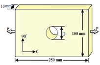
The geometry and default dimensions of the problem are shown in Figure 1. The starting point of applying a continuous mechanical model to a multilayer composite is to examine a multilayer layer in plane stress state and determine the effective stress.
$\left\{\overline{\sigma\}}=\left\{\frac{\left\langle\sigma_{11}\right\rangle+}{\left(1-\mathrm{d}_{1}\right)}+\left\langle\sigma_{11}\right\rangle-\frac{\left\langle\sigma_{22}\right\rangle+}{\left(1-\mathrm{d}_{2}\right)}+\left\langle\sigma_{22}\right\rangle-\frac{\sigma_{12}}{\left(1-\mathrm{d}_{6}\right)}\right\}\right.$ (1)
The effective stress is the applied stress on the degraded surface that effectively resists forces. Parameters $\mathrm{d}_{1} \cdot \mathrm{d}_{2} \cdot \mathrm{d}_{6}$ specifies the degradation status for the three types of stress loading, $\mathrm{d}_{\mathrm{i}}$ between zero (is the healthy) and one (degradable material) [15].
Figure 1. Dimensions and geometry of the problem
2.2 Effective response
The linear elastic compound equation for the degraded material is written in accordance with the principle of equivalent strain [16]. The elastic composite equations for an orthotropic degraded material are as follows [15]:
$\varepsilon_{11}^{E}=\frac{\left\langle\sigma_{11}\right\rangle+}{E_{1}^{0}\left(1-\mathrm{d}_{1}\right)}+\frac{\left\langle\sigma_{11}\right\rangle-}{E_{1}^{0}}-\frac{v_{12}^{0}}{E_{1}^{0}} \sigma_{22}$
$\varepsilon_{22}^{E}=\frac{\left\langle\sigma_{22}\right\rangle+}{E_{2}^{0}\left(1-\mathrm{d}_{2}\right)}+\frac{\left\langle\sigma_{22}\right\rangle-}{E_{2}^{0}}-\frac{v_{12}^{0}}{E_{1}^{0}} \sigma_{11}$
$\varepsilon_{12}^{E}=\frac{\left\langle\sigma_{12}\right\rangle}{2 G_{12}^{0}\left(1-\mathrm{d}_{6}\right)}$ (2)
Based on the laboratory results for some materials, as well as the values $\frac{v_{12}}{E_{1}}=\frac{v_{12}^{0}}{E_{1}^{0}}=\frac{v_{21}^{0}}{E_{2}^{0}}$ in order to remain constant throughout evolution it has been destroyed. In Eq. (2) answers in modulus $G_{12} \cdot E_{2} \cdot E_{1}$ from the degraded layer it is shown that in terms of parameters $d_{6} . d_{2} . d_{1}$ and $G_{12}^{0} . E_{2}^{0} . E_{1}^{0}$ modules are unmodified material [11]
$\begin{aligned} E_{1} &=E_{1}^{0}\left(1-d_{1}\right) \\ E_{2} &=E_{2}^{0}\left(1-d_{2}\right) \\ E_{12} &=E_{12}^{0}\left(1-d_{6}\right) \end{aligned}$ (3)
2.3 Thermodynamic forces
Thermodynamic forces $Y_{6} . Y_{2} . Y_{1}$ Which give the variables of internal degradation and elastic strain energy density $E_{D}$ dependent in the current state of stress and degradation; the partial derivative can be shown below [15]:
$Y_{1}=\frac{\partial E_{D}}{d_{1}}\left|\bar{\sigma} \cdot d_{2} \cdot d_{6}: \operatorname{cons}\right|$
$Y_{2}=\frac{\partial E_{D}}{d_{2}}\left|\bar{\sigma} \cdot d_{1} \cdot d_{6}: \operatorname{cons}\right|$
$Y_{6}=\frac{\partial E_{D}}{d_{6}}\left|\bar{\sigma} \cdot d_{1} \cdot d_{2}: \operatorname{cons}\right|$ (4)
The average value of the strain energy density of the degraded layers can be written in terms of effective stresses, which is the difference between normal tensile stress and normal compressive stress by brackets.
$E_{D}=\frac{1}{2}\left[\frac{\left\langle\sigma_{11}\right\rangle^{2}+}{E_{1}^{0}\left(1-\mathrm{d}_{1}\right)}+\frac{\left\langle\sigma_{11}\right\rangle^{2}-}{E_{1}^{0}}-2 \frac{v_{12}^{0}}{E_{1}^{0}} \sigma_{11} \sigma_{22}+\frac{\left\langle\sigma_{22}\right\rangle^{2}+}{E_{2}^{0}\left(1-\mathrm{d}_{2}\right)}+\frac{\left\langle\sigma_{22}\right\rangle^{2}-}{E_{2}^{0}}+\frac{\sigma_{12}^{2}}{G_{12}^{0}\left(1-\mathrm{d}_{6}\right)}\right]$ (5)
By placing Eq. (3) in Eq. (4) thermodynamic forces are obtained in terms of stress components and degradation variables:
$Y_{1}=\frac{\partial E_{D}}{d_{1}}\left|\bar{\sigma} \cdot d_{2} \cdot d_{6}: \operatorname{cons}\right|=\frac{\left\langle\sigma_{11}\right\rangle^{2}+}{E_{1}^{0}\left(1-\mathrm{d}_{1}\right)^{2}}$
$Y_{2}=\frac{\partial E_{D}}{d_{2}}\left|\bar{\sigma} \cdot d_{1} \cdot d_{6}: \operatorname{cons}\right|=\frac{\left\langle\sigma_{22}\right\rangle^{2}+}{E_{2}^{0}\left(1-\mathrm{d}_{2}\right)^{2}}$
$Y_{6}=\frac{\partial E_{D}}{d_{6}}\left|\bar{\sigma} \cdot d_{1} \cdot d_{2}: \operatorname{cons}\right|=\frac{\left\langle\sigma_{12}\right\rangle^{2}+}{G_{12}^{0}\left(1-\mathrm{d}_{6}\right)}$ (6)
2.4 Evolution of destruction
A particular form of the law of evolution of degradation is in the matter of Ladeveze theory of matter. This model has been proven for highly orthotropic composites such as carbon/epoxy. Initially, a test for carbon/epoxy was established, which is mostly for continuous fiber composites. Damages other than fiber breakage do not cause modulus loss in the fiber direction, so in the absence of fiber breakage $d_{1}$ is zero and at plate stresses only $Y_{2}$ and $Y_{6}$ thermodynamic forces are present. $Y_{2}$ and $Y_{6}$ The maximum amount of thermodynamic force obtained outside the loading path $\tau \leq t$ for each $\tau$ Bigger than the current time [15]:
$Y_{2}(t)=\max \left\{Y_{2}(\tau)\right\} \quad T \leq t$ (7)
$Y_{6}(t)=\max \left\{Y_{6}(\tau)\right\} \quad \tau \leq t$ (8)
Then the linear combination of $Y_{2}$ and $Y_{6}$:
$Y=\left(Y_{6}+b Y_{2}\right)$ (9)
b, it is a matter-dependent constant that indicates the coupling effect between transverse tensile and shear. $Y,$ a simple linear combination of effective thermodynamic forces. Eventually $Y$ maximum $Y$ for each $\tau$ larger than currently introduced.
$Y(t)=\max \left\{Y_{6}(\tau)+b Y_{2}(\tau)\right\} \quad T \leq t$ (10)
Laboratory results for highly orthotropic composites such as carbon / epoxy under quasi-static shear loading have shown that the degradation evolution law for $d_{6}$ :
$d_{6}=\frac{\langle\sqrt{Y-\sqrt{Y_{0}}\rangle}+}{\sqrt{Y_{c}}}$ (11)
Laboratory results for carbon/epoxy also show the degradation evolution law for transverse tensile loading as follows [15]:
$d_{2}=\frac{\langle\sqrt{Y-\sqrt{\tilde{Y}_{0}}}\rangle+}{\sqrt{\tilde{Y}_{c}}}$ (12)
Parameters $\tilde{Y}_{0} \cdot \tilde{Y}_{c} \cdot Y_{c} \cdot Y_{0}$ and b constants are the material through the testing for the composite IM6/914 the properties of which are given in Table 2 specified, and the Table 3 specified. The thickness of each layer is 0.125 mm.
Table 2. IM6/914 composite the properties [15]
$$\begin{array}{|c|c|c|c|c|}
\hline \mathbf{E}_{1}(\mathbf{G P a}) & \mathbf{E}_{2}(\mathbf{G P a}) & \mathbf{E}_{12}(\mathbf{G P a}) & \mathbf{V}_{12} & \mathbf{V}_{13} \\
\hline 170 & 10.8 & 5.8 & 0.34 & 0.4 \\
\hline
\end{array}$$
Table 3. Constant material parameters [15]
$$\begin{array}{|c|c|c|c|c|}
\hline \tilde{\mathbf{Y}}_{\mathbf{0}}(\mathbf{M P a}) & \tilde{\mathbf{Y}}_{\mathbf{c}}(\mathbf{M P a}) & \mathbf{Y}_{\mathbf{0}}(\mathbf{M P a}) & \mathbf{Y}_{\mathbf{c}}(\mathbf{M P a}) & \mathbf{b} \\
\hline 0.0576 & 14.29 & 0.0225 & 7.673 & 2.5 \\
\hline
\end{array}$$
2.5 Criterion of destruction
The criterion for destruction of transverse traction in each layer can be illustrated as follows:
$\left\{Y_{2} \geq Y_{2}^{c} \quad d_{2}=1\right.$ (13)
And otherwise $d_{2}$ Eq. (9) it is calculated; and can be written for damage in the shear direction
$\left\{Y_{2} \geq Y_{2}^{c} \quad d_{6}=1\right.$ (14)
And otherwise $d_{6}$ Eq. (8) it will be counted. Fragility and degradation thresholds are consistent with the failure of the interface between $Y_{2}^{c}$ and the matrix is due to transverse tensile loading.
At this stage the stresses are calculated for the new constants due to the altered properties due to the drop created in the previous step.
$\left[\begin{array}{c}\sigma_{x} \\ \sigma_{y} \\ \tau_{x y}\end{array}\right]=\left[\begin{array}{ccc}Q_{x x} & Q_{x y} & 0 \\ Q_{x y} & Q_{y y} & 0 \\ 0 & 0 & Q_{s s}\end{array}\right]\left[\begin{array}{c}\varepsilon_{x} \\ \sigma \varepsilon_{y} \\ \gamma_{x y}\end{array}\right]$
$Q_{x x}=\frac{E_{1}}{1-v_{12} v_{21}}$
$Q_{y y}=\frac{E_{2}}{1-v_{12} v_{21}}$
$Q_{s s}=G_{12}$
$Q_{x y}=\frac{v_{12} E_{2} E_{1}}{E_{1}-v_{12}^{2} E_{2}}$
$E_{1}=E_{1}^{0}\left(1-d_{1}\right)$
$E_{2}=E_{2}^{0}\left(1-d_{2}\right)$
$G_{12}=G_{12}^{0}\left(1-d_{6}\right)$ (15)
In solving problems with finite element method, it is necessary to examine the independence of the mesh. To check the independence of the mesh, the mesh size is reduced so that the answer is not much different from the previous answer (according to the required accuracy of the problem), the previous mesh is selected as the optimal mesh. In this paper, the maximum stress is selected for comparison. The results are compared for different sizes of mesh in the Table 3. The dimensions used are as shown in Table 4.
Table 4. Investigating the independence of mesh
$$\begin{array}{|c|c|}
\hline \text { Maximum stress (Mpa) } & \text { Mesh size (mm) } \\
\hline 511.62 & 4 \\
\hline 497.71 & 3 \\
\hline 478.22 & 2 \\
\hline 474.23 & 1 \\
\hline 473.83 & 0.5 \\
\hline
\end{array}$$
Therefore, Structural mesh with size of 1 mm can be the optimal size for the problem. But with this mesh size for the whole geometry, the solution time is extended, Therefore, by using the geometry section tool, this mesh size is used only around the hole. The problem mesh is shown in the Figure 2.
Figure 2. Problem mesh
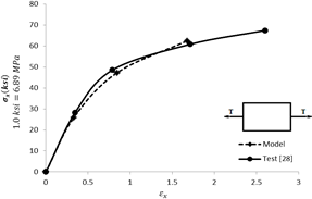
This section presents the validation of the model presented for different lay-up technique. The stress-strain diagram for two different porcelain layers under different loads is presented to investigate the accuracy of the model in predicting the stiffness loss trend and determining the fracture point. Figure 3 shows the Stress–strain curve of the uniaxial tensile for the lay-up technique $[-12 / 78]_{2 s}$ a comparison of the results of the proposed model and the experimental results is given. As can be seen from the figure, the model is slightly conservative at the fracture point stress, which is an advantage in the design of composite structures.
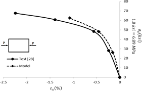
In Figure 4 Stress- strain diagram of the uniaxial pressure for the $[-12 / 78]_{2 s}$ is presented in order to compare the results of the model and the experimental results.
In Figure 5 the stress-strain diagram of the uniaxial tensile for the lay-up technique $[67.5 / 22.5]_{2 s}$ is presented in order to compare the results of the model and the experimental results. The stress has simulated and predicted the fracture point, which demonstrates the model ability to deal with different lay-up technique. This is a very useful and useful feature especially in samples containing stress concentration.
Figure 3. Stress-strain curve under for layer $[-12 / 78]_{2 s}$ tensile loading
Figure 4. Stress-strain curve for layer $[-12 / 78]_{2 \mathrm{s}}$ under pressure loading
Figure 5. Stress-strain curve for layer $
Samples review containing stress concentration from the outputs obtained which Table 5 illustrates the dimensions of the sample.
Table 5. The Dimensions Model
$$\begin{array}{|c|c|c|c|}
\hline \begin{array}{c}
\text { The } \\
\text { Length } \\
\text { (mm) }
\end{array} & \begin{array}{c}
\text { The } \\
\text { Width } \\
\text { (mm) }
\end{array} & \begin{array}{c}
\text { The diameter of } \\
\text { the hole } \\
\text { (mm) }
\end{array} & \begin{array}{c}
\text { The thickness of } \\
\text { each layer } \\
\text { (mm) }
\end{array} \\
\hline 250 & 100 & 40 & 0.125 \\
\hline
\end{array}$$
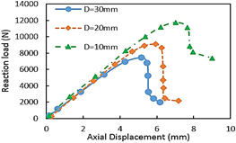
Reaction force and displacement curves is shown in Figure 6.
Figure 6. Reaction force and displacement curves
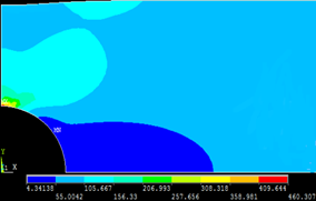
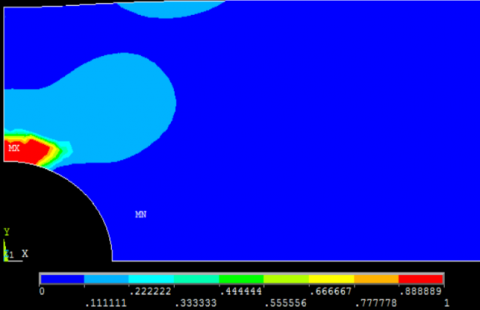
Figure 7. Stress contour x at direction 0° for lay-up technique [0/90]2s
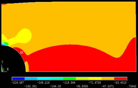
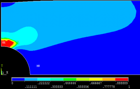
Figure 8. Stress contour x at direction 90° for lay-up technique [0/90]2s
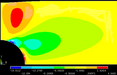
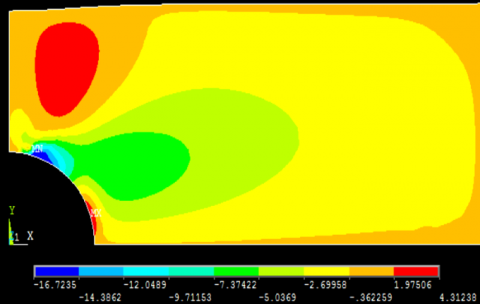
In Figure 7 stress contour x at direction 0° for lay-up technique [0/90]2s and in Figure 8 at layer 90° under 25 MPa loading for lay-up technique [0/90]2s. Figure 9 stress contour y at direction 0° for lay-up technique [0/90]2s and in Figure 10 layer 90° under 25 MPa loading for lay-up technique [0/90]2s.
Figure 9. Stress contour y at direction 0° for lay-up technique [0/90]2s
Figure 10. Stress contour y at direction 90° for lay-up technique [0/90]2s
Figure 11. Stress contour xy at direction 0° for lay-up technique [0/90]2s
Figure 12. Stress contour xy at direction 90° under 25 MPa loading for lay-up technique [0/90]2s
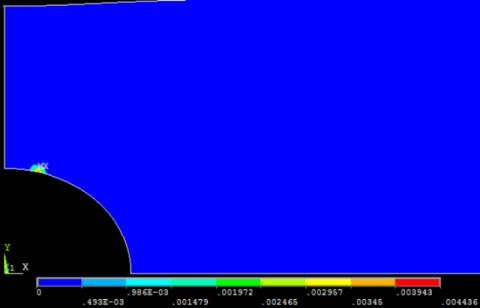
Figure 13. Destruction contour d2 y at direction 0° for lay-up technique [0/90]2s
Figure 14. Destruction contour d2 y at direction 90° for lay-up technique [0/90]2s
Figure 15. Destruction contour d6 y at direction 0° for lay-up technique [0/90]2s
Figure 16. Destruction contour d6 y at direction 90° for lay-up technique [0/90]2s
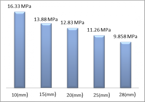
Figure 17. Stress to initiate first degradation in the 0° layer for (d2 = 1 or d6 = 1)
Figure 18. Defined line
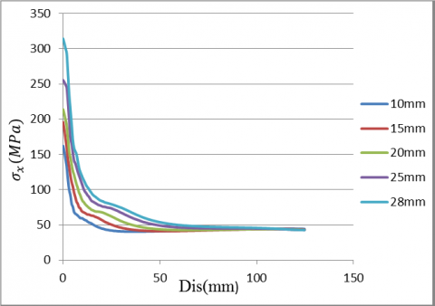
Figure 19. Stress in the x direction 0° layer under 15 MPa load
Figure 20. Stress in the y direction 0° layer under 15 MPa load
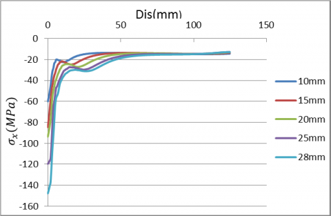
Figure 21. Stress in the x direction 90° layer under 15 MPa load
In Figure 11 stress contour xy at direction 0° for lay-up technique [0/90]2s and in Figure 12 stress contour xy at direction 90° under 25 MPa loading for lay-up technique [0/90]2s. Figure 13 destruction contour d2 y at direction 0° for lay-up technique [0/90]2s and in Figure 14 destruction contour d2 y at direction 90° for lay-up technique [0/90]2s and in Figure 15 destruction contour d6 y at direction 0° for lay-up technique [0/90]2s and in Figure 16 destruction contour d6 y at direction 90° for lay-up technique [0/90]2s.
Figure 17 is shown for five different diameters of the stress segment internal openings, in order to initiate the first degradation (d2 = 1 or d6 = 1), all occurring in the 0° layer. As can be seen from the figure, as the hole diameter decreases the stress tolerance of the specimen decreases in order to form the first degradation. In Figure 18 is shown defined line. In Figure 19 stress in the x direction for five different diameters and in the 0 ° layer calculated under 15 MPa load and the results are compared with each other. In Figure 20 stress in the y direction for five different diameters, and in the layer 0° is calculated under 15 MPa load and compared with each other. In Figure 21 stresses in the x direction for five different diameters and in the 90 ° layer at 15 MPa load are calculated and compared with each other. increasing the diameter increases the maximum stress in the sample.
The results of analyses indicated that the initial damage, progressive damage of the composite laminates, and the strength of the laminates not only depend on the diameter of the holes but also depend on the structure of the composite laminates under the same applied load a condition. According to the model investigated and the finite element solution of the mentioned fragment the following results can be deduced:
[1] Camanho, P.P., Maimí, P., Dávila, C.G. (2007). Prediction of size effects in notched laminates using continuum damage mechanics. Composites Science and Technology, 67(13): 2715-2727. https://doi.org/10.1016/j.compscitech.2007.02.005
[2] Maa, R.H., Cheng, J.H. (2002). A CDM-based failure model for predicting strength of notched composite laminates. Composites Part B: Engineering, 33(6): 479-489. https://doi.org/10.1016/S1359-8368(02)00030-6
[3] Chen, J.F., Morozov, E.V., Shankar, K. (2014). Simulating progressive failure of composite laminates including in-ply and delamination damage effects. Composites Part A: Applied Science and Manufacturing, 61: 185-200. https://doi.org/10.1016/j.compositesa.2014.02.013
[4] Kiral, B.G. (2010). Effect of the clearance and interference-fit on failure of the pin-loaded composites. Materials and Design, 31(1): 85–93. https://doi.org/10.1016/j.matdes.2009.07.009
[5] Mishra, A., Naik, N.K. (2010). Failure initiation in composite structures under low-velocity impact: Analytical studies. Composite Structures, 92(2): 436-444. https://doi.org/10.1016/j.compstruct.2009.08.024
[6] Kapti, S., Sayman, O., Ozen, M., Benli, S. (2010). Experimental and numerical failure analysis of carbon/epoxy laminated composite joints under different conditions. Materials and Design, 31(10): 4933–4942. https://doi.org/10.1016/j.matdes.2010.05.018
[7] Hassan, M.A., Naderi, S., Bushroa, A.R. (2014). Low-velocity impact damage of woven fabric composite: Finite element Simulation and experimental verification. Materials and Design, 53: 706-718. https://doi.org/10.1016/j.matdes.2013.07.068
[8] Rashiddadash, S., Sadighi, M., Dariushi, S. (2018). Experimental and numerical investigation of sandwich panels with bilateral connection under static loading. Journal of Science and Technology of Composites (JSTC), 5(3): 415-426.
[9] Machado, J.J.M., Gamarra, P.R., Marques, E.A.S., da Silva, L.F. (2018). Numerical study of the behaviour of composite mixed adhesive joints under impact strength for the automotive industry. Composite Structures, 185: 373-380. https://doi.org/10.1016/j.compstruct.2017.11.045
[10] Liu, B., Han, Q., Zhong, X., Lu, Z. (2019). The impact damage and residual load capacity of composite stepped bonding repairs and joints. Composites Part B: Engineering, 158: 339-351. https://doi.org/10.1016/j.compositesb.2018.09.096
[11] Petrudi, M.A., Vahedi, K., Kamyab, M.H., Petrudi, M.M.A. (2019). Numerical and experimental study of oblique penetration of blunt projectile into ceramic-aluminum target. Modares Mechanical Engineering, 19(5): 1253-1263.
[12] Tang, M.L., Ao, Y.H., Wang, C., Wang, P.F. (2020). Facile synthesis of dual Z-scheme g-C3N4/Ag3PO4/AgI composite photocatalysts with enhanced performance for the degradation of a typical neonicotinoid pesticide. Applied Catalysis B: Environmental, 268: 118395. https://doi.org/10.1016/j.apcatb.2019.118395
[13] Stephane, L., Ferrer, D., Portoles, J. (2020). Mechanical reinforcement for a part made of composite material, in particular for a wind turbine blade of large dimensions. U.S. Patent 10,544,688, issued January 28. https://patents.google.com/patent/US10544688B2/en, accessed on Jan. 29, 2020.
[14] Ladeveze, P. (1992). A damage computational method for composite structures. Computers & Structures, 44(1-2): 79-87. https://doi.org/10.1016/0045-7949(92)90226-P
[15] Herakovich, C.T. (1998). Mechanics of Fibrous Composites. http://www.sidalc.net/cgibin/wxis.exe/?IsisScript=CICY.xis&method=post&formato=2&cantidad=1&expresion=mfn=003779, accessed on Jan. 29, 2020.
[16] Ribeiro-Ayeh, S. (2005). Finite element modelling of the mechanics of solid foam materials (Doctoral dissertation, KTH). http://www.divaportal.org/smash/record.jsf?pid=diva2%3A7450&dswid=6262, accessed on Jan. 29, 2020.
[17] Pickering, S.J. (2006). Recycling technologies for thermoset composite materials—current status. Composites Part A: Applied Science and Manufacturing, 37(8): 1206-1215. https://doi.org/10.1016/j.compositesa.2005.05.030
[18] Yuanjian, T., Isaac, D.H. (2007). Impact and fatigue behaviour of hemp fibre composites. Composites Science and Technology, 67(15-16): 3300-3307. https://doi.org/10.1016/j.compscitech.2007.03.039
[19] Lemaitre, J. (1971). Evaluation of dissipation and damage in metals. In Proc. ICM (Vol. 1). https://ci.nii.ac.jp/naid/10007808098/, accessed on Jan. 29, 2020.
[20] Talreja, R. (1986). Stiffness properties of composite laminates with matrix cracking and interior delamination. Engineering Fracture Mechanics, 25(5-6): 751-762. https://doi.org/10.1016/0013-7944(86)90038-X