Energy and exergy analysis of flat plate solar collector for three working fluids, under the same conditions

2.1. Energy analysis

Collector’s energy analysis, in order to attain the amount of heat it receives, obtained its efficiency and working fluids outlet temperature is very important.

For this purpose, the climatic conditions of the place where the collector (such as solar radiation received, solar radiation angle, Sunset angle, latitude angle and etc.) is installed must be available.

By knowing the amount of monthly average solar radiation received on the horizontal surface of the earth, monthly average diffuse radiation calculated from the equation 1 [10]:

$\overline{\mathrm{H}}_{\mathrm{d}}=\overline{\mathrm{H}}_{\mathrm{b}}\left(1-1.13 \overline{\mathrm{K}}_{\mathrm{t}}\right)$    (1)

$\overline{\mathrm{H}}_{\mathrm{d}}$ is monthly average diffuse radiation, $\overline{\mathrm{H}}_{\mathrm{b}}$ is monthly average radiation received on the horizontal surface of the ground, $\overline{\mathrm{K}}_{\mathrm{t}}$ is  monthly average clearness index.

To obtain the amount of monthly average absorbed solar radiation by FPC, (2-14) steps are followed.

At first, according to the incident beam angle and FPC glass, refracted beam angle can be calculated from the equation2 [22-23]:

$\mathrm{n}_{1} \cdot \sin \alpha_{\mathrm{i}}=\mathrm{n}_{2} \cdot \sin \theta$    (2)

n₁ and n₂ are refracted index for air and glass respectively, α_i is incident beam angle and θ is refracted beam angle.

Transmittance absorption losses factor is [22-23]:

τ_α = exp($\frac{-\mathrm{KL}}{\cos \theta}$)    (3)

KL is absorbed solar radiation rate for glass

Then transmittance refraction losses factor is [22-23]:

τ_r = $\frac{1}{2}\left(\frac{1-r \|}{1+r \|}+\frac{1-r \perp}{1+r \perp}\right)$        (4)

In this equation $\mathbf{r}_{ \|}$ and $\mathrm{r}_{\perp}$ are parallel and perpendicular component of unpolarized radiation respectively and can be calculated from equations 5 and 6 [22-23]:

$\mathbf{r}_{ \|}=\frac{\tan ^{2}(\theta-\alpha)}{\tan ^{2}(\theta+\alpha)}$        (5)

$r_{\perp}=\frac{\sin ^{2}(\theta-\alpha)}{\sin ^{2}(\theta+\alpha)}$        (6)

Therefore, transmittance factor for glass is [22-23]:

τ = τ_α × τ_r    (7)

At this step, absorptance factor can be found from the properties of the absorber, which is [22-23]:

$\frac{\alpha_{\mathrm{B}}}{\alpha_{\mathrm{n}}}=1+2.0345 \times 10^{-3} \alpha-1.99 \times 10^{-4} \alpha^{2}+5.324 \times$$10^{-6} \alpha^{3}-4.799 \times 10^{-8} \alpha^{4}$    (8)

$\alpha_{\mathrm{n}}$ is absorptance factor at normal incident can be found from the properties of the absorber. 

The amount of effective product transmittance –absorptance that finally absorbs the absorber is [22]:

$(\tau \alpha)_{\mathrm{B}}=(1.01 \tau) . \alpha_{\mathrm{B}}$    (9)

For given collector tilted angle (β), the effective incidence angle for diffuse radiation from sky and effective incidence angle for ground reflected radiation, can be calculated from equations 10 and 11 respectively [22-23]:

$\theta_{\mathrm{e}, \mathrm{D}}=59.68-0.1388 \beta+0.001497 \beta^{2}$    (10)

$\theta_{\mathrm{e}, \mathrm{G}}=90-0.5788 \beta+0.00269 \beta^{2}$    (11)

By placing $\theta_{\mathrm{e}, \mathrm{D}}$ and $\theta_{\mathrm{e}, \mathrm{G}}$ in the  equation 2 and solving  equations number 2 to 9, the effective product transmittance – absorptance that finally will be diffused and the effective product transmittance – absorptance that finally reflected from the ground can be calculated from  equations 12 and 13 respectively [22-23]:

$(\tau \alpha)_{\mathrm{D}}=(1.01 \tau) . \alpha_{\mathrm{D}}$    (12)

$(\tau \alpha)_{\mathrm{G}}=(1.01 \tau) . \alpha_{\mathrm{G}}$    (13)

Table 1. Flat plate solar collector features

Therefore, monthly average absorbed solar radiation by FPC is [22-23]:

$\overline{\mathrm{S}}=\overline{\mathrm{H}}_{\mathrm{b}} \cdot \overline{\mathrm{R}}_{\mathrm{b}} \cdot (\tau \alpha)_{\mathrm{B}}+(\mathrm{\tau} \alpha)_{\mathrm{D}} \cdot\left(\frac{1+\cos \beta}{2}\right) \cdot \overline{\mathrm{H}}_{\mathrm{d}}$$+\rho_{\mathrm{G}} .(\tau \alpha)_{\mathrm{G}} \cdot\left(\frac{1-\cos \beta}{2}\right) \cdot\left(\overline{\mathrm{H}}_{\mathrm{b}}+\overline{\mathrm{H}}_{\mathrm{d}}\right)$    (14)

$\overline{\mathrm{R}}_{\mathrm{b}}$ is monthly beam radiation tilt factor, ρ_G is ground reflectance factor.

Monthly average total solar radiation is [22-23]:

$\overline{\mathrm{I}}_{\mathrm{t}}=\frac{\overline{\mathrm{s}}}{(\mathrm{\tau} \alpha) \mathrm{ave}}$    (15)

$(\tau \alpha)_{\text { ave }}$ is average effective product transmittance – absorptance and can be calculated from equation16 [22-23]:

$(\tau \alpha)_{\mathrm{ave}}=0.96(\tau \alpha)_{\mathrm{B}}$    (16)

By calculated overall heat loss coefficient, the rate of useful energy collected from FPC and FPC’s efficiency obtained. overall heat loss coefficient, include three terms:

1. top loss coefficient [15]:

$\mathrm{U}_{\mathrm{t}}=\frac{1}{\frac{\mathrm{Ng}}{\frac{\mathrm{C}}{\mathrm{T} \mathrm{p}}\left(\frac{\mathrm{T}_{\mathrm{p}}-\mathrm{T}_{\mathrm{a}}}{\mathrm{N} \mathrm{g}+\mathrm{f}}\right)^{0.33}+\frac{1}{\mathrm{h}_{\mathrm{W}}}}}$            （17）

N_g is number of glass cover, T_p is mean absorber temperature, T_a is ambient air temperature, h_w is wind convection heat loss coefficient, C and f are constant parameters [15].

$\mathrm{h}_{\mathrm{w}}=\frac{8.6 \mathrm{V}^{0.6}}{\mathrm{L}^{0.4}}$    (18)

$\mathrm{C}=365.9\left(1-0.00883 \beta+0.0001298 \beta^{2}\right)$    (19)

$\mathrm{f}=\left(1-0.04 \mathrm{h}_{\mathrm{w}}+0.0005 \mathrm{h}_{\mathrm{w}}^{2}\right)\left(1+0.091 \mathrm{N}_{\mathrm{g}}\right)$    (20)

2. bottom heat loss coefficient [22]:

$\mathrm{U}_{\mathrm{b}}=\frac{1}{\frac{\mathrm{tb}}{\mathrm{k}_{\mathrm{b}}}+\frac{1}{\mathrm{h}_{\mathrm{c}, \mathrm{b}-\mathrm{a}}}}$            (21)

t_b is thickness of back insulation, h_c,b-a is convection heat loss coefficient from back to ambient, K_b is conductivity of back insulation.

3. heat loss coefficient from the collector edge [22]:

$\mathrm{U}_{\mathrm{e}}=\frac{1}{\frac{\mathrm{t}_{\mathrm{e}}}{\mathrm{k}_{\mathrm{e}}}+\frac{1}{\mathrm{h}_{\mathrm{c}, \mathrm{e}-\mathrm{a}}}}$            (22)

t_e is thickness of edge insulation, h_c,e-a  is convection heat loss coefficient from edge to ambient, K_e is conductivity of edge insulation.

Therefore, overall heat loss coefficient is [11-12]:

U_L = U_t + U_e + U_b                                                               (23)

The useful heat gain by the working fluid is [1]:

$\mathrm{Q}_{\mathrm{u}}=\dot{\mathrm{m}} \cdot \mathrm{C}_{\mathrm{p}} \cdot\left(\mathrm{T}_{\mathrm{out}}-\mathrm{T}_{\mathrm{in}}\right)$    (24)

$\dot{\mathrm{m}}$ is working fluid mass rate, Cp is heat capacity, T_out and T_in are outlet and inlet temperature respectively.

The useful heat gain of FPC system, considering the heat losses from the FPC to the atmosphere, is [11,22]:

$\mathrm{Q}_{\mathrm{u}}=\mathrm{A}_{\mathrm{c}}\left[\mathrm{G}_{\mathrm{t}}(\tau \alpha)-\mathrm{U}_{\mathrm{L}}\left(\mathrm{T}_{\mathrm{p}}-\mathrm{T}_{\mathrm{a}}\right)\right]$    (25)

A_c is collector area, G_t is total solar radiation.

Collector's performance, collector efficiency and collector efficiency factor calculated from equations 27 and 28 [11]:

$\eta=\frac{\mathrm{Qu}}{\mathrm{A}_{\mathrm{C}} \cdot \mathrm{G}_{\mathrm{t}}} \times 100$    (26)

$\mathrm{F}_{\mathrm{C}}=\frac{\frac{1}{\mathrm{U}_{1}}}{\mathrm{W}_{\mathrm{i}}\left[\frac{1}{\mathrm{U}_{1} \cdot\left(\mathrm{D}+\left(\mathrm{W}_{\mathrm{i}}-\mathrm{D}\right) \cdot \mathrm{F}_{\mathrm{f}}\right)}+\frac{1}{\mathrm{C}_{\mathrm{b}}}+\frac{1}{\mathrm{\pi} \cdot \mathrm{D}_{\mathrm{i}} \cdot \mathrm{h}_{\mathrm{fi}}}\right]}$               (27)

W_i is tubes spacing, D is tube outside diameter, D_i is tube inside diameter, h_fi is heat transfer coefficient inside of the tube, F_f is fin efficiency, C_b is bond conductance.

Fin efficiency is [22-23]:

$\mathrm{F}_{\mathrm{f}}=\frac{\tanh \left(\mathrm{X}\left(\frac{\mathrm{w}_{\mathrm{i}-\mathrm{D}}}{2}\right)\right)}{\mathrm{x}\left(\frac{\mathrm{W}_{\mathrm{i}}-\mathrm{D}}{2}\right)}$            (28)

X is a constant parameter and equal to [22-23]:

$X=\left[\frac{U_{1}}{K \delta_{t}}\right]$    (29)

Plate’s material is copper. K is plate heat transfer coefficient, $\delta_{\mathrm{t}}$ is plate thickness.

Bond conductance can be calculated from equation 31 [22-23]:

$\mathrm{C}_{\mathrm{b}}=\frac{\mathrm{K}_{\mathrm{b}} \cdot \mathrm{b}}{\gamma}$    (30)

K_b is bond thermal conductivity, b is bond width, γ is bond thickness.

The fluid outlet temperature has a very important role in collector systems. In FPC it is equal to [9]:

$\mathrm{T}_{\mathrm{out}}=\mathrm{T}_{\mathrm{in}}+\left[\frac{1}{\mathrm{U}_{1}}\left(\overline{\mathrm{S}}_{\mathrm{w}}-\mathrm{U}_{1}\left(\mathrm{T}_{\mathrm{in}}-\mathrm{T}_{\mathrm{a}}\right)\right)\right]$$\cdot\left[1-\exp \left(\frac{-\mathrm{A}_{\mathrm{c}} \cdot \mathrm{U}_{\mathrm{L}} \cdot \mathrm{F}_{\mathrm{c}}}{\dot{\mathrm{m}} \cdot \mathrm{C}_{\mathrm{p}}}\right)\right]$    (31)

$\overline{\mathrm{S}}_{\mathrm{w}}$ is average absorbed solar radiation in (W/m²) [22]

$\overline{\mathrm{S}}_{\mathrm{w}}=\frac{\overline{\mathrm{G}}_{\mathrm{t}}}{(\tau \alpha) \mathrm{ave}}$    (32)

2.2 Exergy analysis

Exergy analysis is a method that use the second law of thermodynamics for the analysis, design and improvement of energy. Exergy is defined as the maximum amount of power which can be produced by a system and has an important role in thermodynamic analysis.

Exergy analysis for a control volume can be calculated from equation 34 [24]:

$\frac{\mathrm{dEX}_{\mathrm{cv}}}{\mathrm{dt}}=\sum_{\mathrm{j}}\left(1-\frac{\mathrm{T}_{0}}{\mathrm{T}_{\mathrm{j}}}\right) \dot{\mathrm{Q}}_{\mathrm{j}}-\left(\dot{\mathrm{W}}_{\mathrm{cv}}-\mathrm{P}_{0} \frac{\mathrm{d} \mathrm{V}_{\mathrm{cv}}}{\mathrm{dt}}\right)+$$\sum \dot{\mathrm{m}}_{\mathrm{i}} \mathrm{EX}_{\mathrm{i}}-\sum \dot{\mathrm{m}}_{\mathrm{e}} \mathrm{EX}_{\mathrm{e}}-\dot{\mathrm{EX}}_{\mathrm{d}}$    (33)

When FPC system is in a steady state, exergy balance is [2,14]:

$\dot{\mathrm{EX}}_{\mathrm{in}}-\dot{\mathrm{EX}}_{\mathrm{out}}-\dot{\mathrm{EX}}_{\mathrm{L}}-\dot{\mathrm{EX}}_{\mathrm{d}}=0$    (34)

1.inlet exergy: 

Exergy flows into a system includes two terms, inlet exergy with mass flow and inlet exergy with solar radiation absorbed by the collector.

a. Inlet exergy with mass flow is [2,11]:

$\dot{\mathrm{EX}}_{\mathrm{in}, \mathrm{f}}=\dot{\mathrm{m}} \cdot \mathrm{C}_{\mathrm{p}}\left(\mathrm{T}_{\mathrm{in}}-\mathrm{T}_{\mathrm{a}}-\left(\mathrm{Ta} \ln \frac{\mathrm{T}_{\mathrm{in}}}{\mathrm{T}_{\mathrm{a}}}\right)\right)+\frac{\dot{\mathrm{m}} \Delta \mathrm{P}_{\mathrm{in}}}{\rho}$    (35)

$\Delta \mathrm{P}_{\mathrm{in}}$ is the pressure difference of the working fluid with the surroundings at FPC’s inlet.

b. Inlet exergy with solar radiation absorbed by the collector is [4]:

$\dot{\mathrm{EX}}_{\mathrm{in}, \mathrm{q}}=\eta_{\mathrm{o}} . \mathrm{G}_{\mathrm{t}} \cdot \mathrm{A}_{\mathrm{c}}\left(1-\frac{\mathrm{T}_{\mathrm{a}}}{\mathrm{T}_{\mathrm{S}}}\right)$    (36)

T_s is Apparent solar temperature, η_o is optical efficiency and equal to [15,16]:

η_o $=\frac{\overline{\mathrm{S}}}{\overline{\mathrm{I}}_{\mathrm{t}}}$    (37)

Thus, inlet exergy is [2-3]:

$\dot{\mathrm{EX}}_{\mathrm{in}}=\dot{\mathrm{EX}}_{\mathrm{in}, \mathrm{f}}+\dot{\mathrm{EX}}_{\mathrm{in}, \mathrm{q}}$    (38)

2. outlet exergy:

The outlet exergy includes only the outlet exergy with mass flow and equal to [2,7]:

$\dot{\mathrm{EX}}_{\mathrm{out}}=\dot{\mathrm{m}} \cdot \mathrm{C}_{\mathrm{p}}\left(\mathrm{T}_{\mathrm{out}}-\mathrm{T}_{\mathrm{a}}-\left(\mathrm{Ta} \ln \frac{\mathrm{T}_{\mathrm{out}}}{\mathrm{T}_{\mathrm{a}}}\right)\right)+\frac{\dot{\mathrm{m}} \cdot \Delta \mathrm{P}_{\mathrm{out}}}{\rho}$    (39)

$\Delta \mathrm{P}_{\mathrm{out}}$ is the pressure difference of the working fluid with the surroundings at FPC’s outlet.

3. Leakage exergy

Includes heat leakage from the absorber plate to the environment. The outlet exergy is the desired exergy and the exergy leakage equals the undesired exergy losses.

$\dot{\mathrm{EX}}_{\mathrm{L}}=\mathrm{U}_{\mathrm{L}} \cdot \mathrm{A}_{\mathrm{c}}\left(\mathrm{T}_{\mathrm{p}}-\mathrm{T}_{\mathrm{a}}\right)\left(1-\frac{\mathrm{T}_{\mathrm{a}}}{\mathrm{T}_{\mathrm{p}}}\right)$    (40)

4. Destruction exergy:

Destruction exergy includes three terms which is discussed below.

a. Destruction exergy due to pressure drop of inside the tube [2,26]:

$\dot{\mathrm{EX}}_{\mathrm{d}, \Delta \mathrm{P}}=\left(\frac{\dot{\mathrm{m}} \Delta \mathrm{P}}{\rho}\right)\left(\frac{\mathrm{T}_{\mathrm{a}} \ln \frac{\mathrm{T}_{\mathrm{out}}}{\mathrm{Ta}}}{\mathrm{T}_{\mathrm{out}}-\mathrm{T} \mathrm{in}}\right)$    (41)

$\Delta \mathrm{P}=\rho \cdot \mathrm{g} \cdot \left(\mathrm{L}_{\mathrm{r}} \cdot \sin \beta+\mathrm{h}_{1}\right)$    (42)

g is gravity acceleration, L_r is tube length, h₁ is total pressure drop and equal to [26]:

$\mathrm{h}_{1}=\frac{8 \cdot \dot{\mathrm{m}}^{2}}{\mathrm{n}_{\mathrm{r}} \cdot \mathrm{g} \cdot \rho^{2} \cdot \pi^{2} \cdot \mathrm{D}_{\mathrm{i}}^{4}}\left(\mathrm{f} \frac{\mathrm{L} \mathrm{r}}{\mathrm{D}_{\mathrm{i}}}+\sum_{\mathrm{i}=1}^{\mathrm{n}_{\mathrm{r}}} \mathrm{K}_{\mathrm{L}}\right)$    (43)

n_r is number of tube, KL is partial pressure drop coefficient of connections that in tube’s inlet equal to 1 and at outlet equal to 0.5, f is friction coefficient and obtained from equation 45 [25]:

$\left\{\begin{array}{ll}{\mathrm{f}=\frac{64}{\mathrm{Re}}} & {\text { laminar flow }} \\ {\mathrm{f}=\frac{0.079}{\mathrm{Re}^{0.25}}} & {\text { turbulent flow }}\end{array}\right.$    (44)

b. Destruction exergy due to solar temperature difference with absorber plate surface [2-3]:

$\dot{\mathrm{EX}}_{\mathrm{d}, \Delta \mathrm{T}_{\mathrm{S}}}=\eta_{\mathrm{o}} \cdot \mathrm{G}_{\mathrm{t}} \cdot {\mathrm{A}_{\mathrm{p}}} \cdot \mathrm{T}_{\mathrm{a}} \cdot\left(\frac{1}{\mathrm{T}_{\mathrm{p}}}-\frac{1}{\mathrm{T}_{\mathrm{S}}}\right)$    (45)

c. Destruction exergy due to the temperature difference between absorber plate surface and working fluid that is [2,7]:

    $\dot{\mathrm{EX}}_{\mathrm{d}, \Delta \mathrm{P}_{\mathrm{f}}}=\dot{\mathrm{m}} \cdot \mathrm{C}_{\mathrm{p}} \cdot \mathrm{T}_{\mathrm{a} \cdot}\left(\ln \frac{\mathrm{T}_{\mathrm{out}}}{\mathrm{T}_{\mathrm{in}}}-\frac{\mathrm{T}_{\mathrm{out}}-\mathrm{T}_{\mathrm{in}}}{\mathrm{T}_{\mathrm{p}}}\right)$

=$1-\left\{\left(1-\eta_{O}\right)+\frac{\dot{m} \Delta P}{\rho G_{t}\left(1-\frac{T_{a}}{T_{s}}\right)} \frac{T_{a} \ln \left(\frac{T_{o u t}}{T_{a}}\right)}{\left(T_{o u t}-T_{i n}\right)}+\right.$    (46)

Therefore, destruction exergy is [2,3,7]:

$\dot{\mathrm{EX}}_{\mathrm{d}}=\dot{\mathrm{EX}}_{\mathrm{d}, \Delta \mathrm{P}}+\dot{\mathrm{EX}}_{\mathrm{d}, \Delta \mathrm{T}_{\mathrm{S}}}+\dot{\mathrm{EX}}_{\mathrm{d}, \Delta \mathrm{P}_{\mathrm{f}}}$    (47)

By doing the balance of exergy, exergy efficiency to understand the FPC performance is defined, that is [11,15]:

$\eta_{\mathrm{EX}}$=$\frac{\dot{\mathrm{m}}\left[\mathrm{C}_{\mathrm{p}}\left(\mathrm{T}_{\mathrm{out}}-\mathrm{T}_{\mathrm{in}}-\left(\mathrm{T}_{\mathrm{a}} \cdot \ln \frac{\mathrm{T}_{\mathrm{out}}}{\mathrm{T}_{\mathrm{i}}}\right)\right)-\frac{\Delta \mathrm{P}}{\rho}\right]}{\mathrm{G}_{\mathrm{t}} \cdot \mathrm{A}_{\mathrm{p}} \cdot\left(1-\frac{\mathrm{T} \mathrm{a}}{\mathrm{T}_{\mathrm{S}}}\right)}$$=$$1-\left\{\left(1-\eta_{O}\right)+\frac{\dot{m} \Delta P}{\rho G_{t}\left(1-\frac{T_{a}}{T_{s}}\right)} \frac{T_{a} \ln \left(\frac{T_{o u t}}{T_{a}}\right)}{\left(T_{o u t}-T_{i n}\right)}+\right.$$\frac{\eta_{O} T_{a}}{\left(1-\frac{T_{a}}{T_{S}}\right)}\left(\frac{1}{T_{P}}-\frac{T_{a}}{T_{s}}\right)+\frac{U_{l}\left(T_{P}-T_{a}\right)}{G_{t}\left(1-\frac{T_{a}}{T_{S}}\right)}\left(1-\frac{T_{a}}{T_{P}}\right)+$$\frac{\dot{m} C_{P} T_{a}}{G_{t} A_{c}} \frac{\left(\ln \left(\frac{T_{o u t}}{T_{i n}}\right)-\frac{\left(T_{o u t}-T_{i n}\right)}{T_{P}}\right)}{\left(1-\frac{T_{a}}{T_{S}}\right)} \}$    (48)

In this study, for a flat plate solar collector that its features are defined, by using three fluids that are water, air and TiO₂ Nano-fluid under the same condition energy and exergy equations are modeling and solving.

As it seen in table 4 the values obtained from energy analysis are reported:

Table 4. Energy analysis result for FPC

1.png

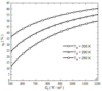
Figure 1. Effects of ambient temperature to FPC efficiency at variable total solar radiation.

As it seen in fig. 1, effect of ambient temperature is shown in the total solar radiation range between 500-1200 Watts. It can be interpreted that efficiency of FPC is directly related to ambient temperature So that, by increasing ambient temperature and total solar radiation FPC Efficiencies increases. Approximately FPC Efficiencies at an appropriate collector tilt angle and working fluid mass flow rate during the year is between 45 % – 55% that is a suitable range.

As it seen in fig. 2, for working fluids that its inlet temperature is between 290 – 320 kelvins, outlet temperature is obtained. TiO₂ Nano-fluid has the highest outlet temperature that its outlet temperature approximately (70-80) ℃ higher than water and (30-40) ℃ higher than air. therefore, Nano-fluids has the more ability than other working fluids.

2.png

Figure 2. Working fluids outlet temperature, based on their inlet temperature

3.png

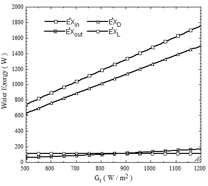
Figure 3. Exergy of water, based on total solar radiation

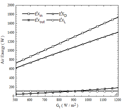
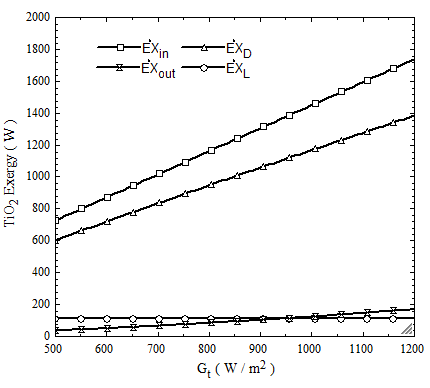
In fig.3, fig.4 and fig.5 effect of total radiation on working fluids exergy, in range between 500-1200 (W/m²) is discussed.

According to the obtained diagrams, when total solar radiation is increasing, exergy increases. Destruction exergy is very affected from solar radiation when ambient temperature is constant. Inlet exergy of working fluids is very higher than outlet exergy.

4.png

Figure 4. Exergy of TiO₂ Nano-fluid, based on total solar radiation

Generally, inlet exergy is between 700-1700 watts, outlet exergy is between 80-200 watts, leakage exergy is between 100-150 watts and destruction exergy is between 600-1400 watts. Exergy of TiO₂ Nano-fluid in the same condition is higher than air, and water has the least exergy.

5.png

Figure 5. Exergy of air Nano-fluid, based on total solar radiation

6.png

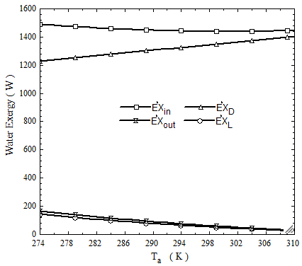
Figure 6. Exergy of water, based on ambient temperature

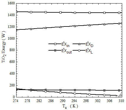
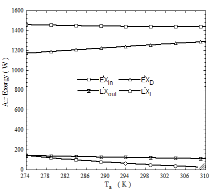
As it seen in fig. 6, fig. 7 and fig. 8 effect of ambient temperature on working fluids exergy, in range between 274-310 kelvins is discussed.

As the ambient temperature increases, the inlet exergy decreases, which water has the most changes and TiO₂ Nano-fluids gives the slightest changes in these conditions.

Generally, the range of exergy changes for inlet exergy is between 1400-1500 watts, for outlet exergy is between 180-20 watts, for leakage exergy is between 180-20 watts. But destruction exergy increases and its changes is between 1200-1450 watts.

7.png

Figure 7. Exergy of TiO₂ Nano-fluid, based on ambient temperature

8.png

Figure 8. Exergy of air, based on ambient temperature

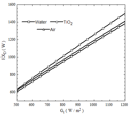
As it seen in fig. 9, destruction exergy of water, more than other two fluids.

Also, the destroyed exergy of the TiO₂ Nano-fluid has the lowest value. Therefore, the use of Nano-fluids is more efficient.

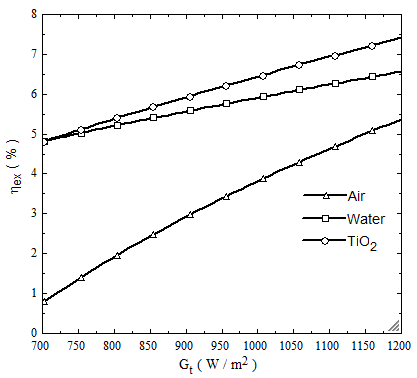
In fig. 10, exergy efficiency based on total solar radiation that is between 700-1200 (W/m²) has been shown. By increasing total solar radiation, the exergy efficiency is rising for all three working fluids. However, the increase in total solar radiation has a great impact on exergy efficiency of TiO₂ Nano-fluid.

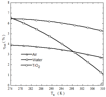
In fig. 12, the effect of the ambient temperature on the exergy efficiency of the working fluids is shown. By increasing ambient temperature, the exergy efficiency is decreased, that water has the most negative variations in exergy efficiency under the same condition. In this state, TiO₂ Nano-fluid also has the highest exergy efficiency.

9.png

Figure 9. Compare destruction exergy of working fluids, based on total solar radiation

10.png

Figure 10. Compare exergy efficiency of working fluids, based on total solar radiation

11.png

Figure 11. Compare exergy efficiency of working fluids, based on ambient temperature

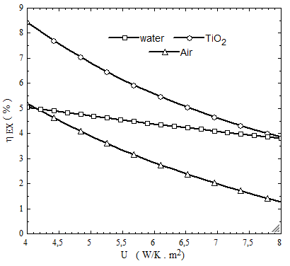
In fig. 12, The effect of increasing the overall heat loss coefficient on the exergy efficiency is shown. As it increases, gradually decreases the exergy efficiency.

In this state, the TiO₂ Nano-fluid is more susceptible to overall heat loss than the other two fluids.

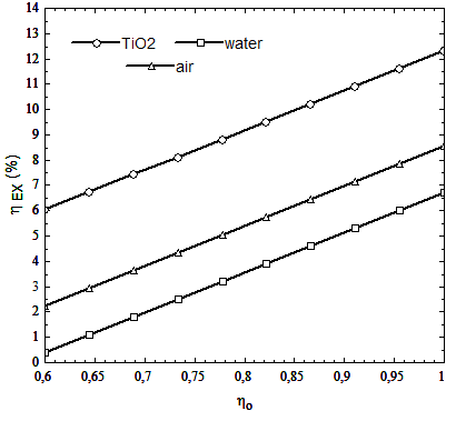
In fig. 13, the effect of exergy efficiency on the optical efficiency is shown. It is observed that the TiO₂ Nano-fluid is more sensitive than other two fluids.

12.png

Figure 12. Compare exergy efficiency of working fluids, based on overall heat loss coefficient

13.png

Figure 13. Compare exergy efficiency of working fluids, based on overall optical efficiency