Sudha Ganesan![]() | Ganesan Kandasamy*
| Ganesan Kandasamy*![]()
© 2023 IIETA. This article is published by IIETA and is licensed under the CC BY 4.0 license (http://creativecommons.org/licenses/by/4.0/).
OPEN ACCESS
In Critical Path Method (CPM), the project managers usually use three quantities; earliest start, latest start and job float for project networking problems. However, interval parameters are used for project scheduling problems dealing with the uncertainties. In this paper, we suggest a new approach for computing the interval time duration of a project networking problem without transforming to crisp equivalent forms. First the interval parameters are represented in their midpoint width form. A new type of arithmetic operations and ranking are applied on the midpoint width form of interval numbers, earliest start, latest start, earliest finish, latest finish and float time are calculated. Interval critical path is identified and the project completion tine is arrived. Numerical description is supplied to describe the method proposed in depth and the results obtained are compared with the existing methods.
Critical Path Method (CPM), interval numbers, interval ranking, interval arithmetic, decision making
A critical path of project management involves certain activities that have to be performed in a specific order and for a certain period. When a member of one task can be dampened or postponed, such a function is then not necessary for a term without losing work on others. Though activities can't wait with a critical value there are time limits during project execution.
Critical Path Method (CPM) is an algorithm for the timing of a project to be prepared, controlled and analysed. The step by phase- CPM process assists to define essential and uncritical research that remove temporary threats from project start to finish. The essential functions include a buffer with a zero-run-time. The parameters of the entire project "change" as the duration of these operations changes. That's why critical project management tasks need careful monitoring and timely recognition of risks.
One American corporation invented the process in 1957. The workers have decided to close down, repairing and restarting chemical services. The roles involved in this project were multiple and dynamic ventures, and that is why a tool like this was required. Critical approach to the path was then spread quickly to agrarian and in building programs where people wished to learn how to reduce repeated behaviour. Today, the approach is widely used to describe critical activities in many fields, including software development.
Benefits of an analysis of critical paths
Evaluation of the critical path is needed to predict timing for completion of the project.
Below are 6 big benefits of CPM:
Which are the critical path system limits?
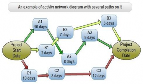
The approach for routine and complex projects is believed to have been established with the goal of a small increase in the delivery time of the tasks. CPM is losing its efficiency to more complicated ventures. There are alternatives to PERT-diagrams and for example, one that allow you to change the operation’s timing. A Critical way limits events and actions within a project in progress, displaying them in a network connected as interconnections as in Figure 1. Activities are known to be node; arches and lines between nodes serve as the beginning and ending of activities.
Figure 1. Critical path from starting point to ending point
The CPM example uses
Find the easiest case in point of a short-term project using critical path technology. Imagine our goal is to arrange a parking of the car near the workplace on an empty asphalted field. Steps to be followed in order to choosing a venue.
It seems clear that, certain phases of this project can't start until the others are finished. They rely on each other. Steps d, e are sequential actions, because they have to take place in some order. In this example, these stages are most common significant crucial duties in trouble solving. You must place them on the project's critical road, since no stages can be started until the others are finished.
It is the cornerstone of strategy, the length is possible to decide the each stage and whole project:
Figures 2 and 3 represent activity network diagrams with several paths on it.
Figure 2. Network diagram of project from starting to completion
Figure 3. Real life example for critical path
CPM Requires 5 Phases in a Row:
1. Identify activities /tasks
Understanding the project's scope, will divide the layout of the work into operations list, assigning names or codes to them. Everything in the planning operations will continue to have a clear time and date.
2. Identify such series
This is the most important pass, as it clearly provides view of the relationships among steps and helps to create relationships, as some acts depends on other acts being carried out.
3. Make your activities a network
If you decided that the behaviours are mutually related, construct a network diagram or a map for the path analysis. Due to their dependencies, tasks can be conveniently linked using the arrows.
4. Determine time intervals for any operation to be completed
Estimate how much time will spend on the job, you should be able to calculate the amount of time it takes to complete the project as a whole (small tasks can be measured in a few days; more complex activities require a thorough review).
5. Find a critical path
Helps to construct the longest track sequence, or critical track, the operating network will use the following parameters as in Figure 4:
Figure 4. Flow diagram for finding critical path
Asset constraint affects process
This will also face some challenges that can impact projects and create new dependencies by attempting to optimize the benefits of the critical path approach and ensuring the project's continued progress. For example, if the team is suddenly reduced from 10 to 5 members, means that you are faced with resource constraints. The critical path is therefore a necessary resource path, where the resources associated with each operation are an important part of the method. This means that some tasks need to be performed in a particular order, which can lead to delays and thus make the project longer than anticipated.
In today's highly competitive business environment, one of the most sought challenging tasks for any boss who can take on a big project that needs teamwork across the company to sustain strategic objectives such as timely delivery and customization. In determining how to organize all these tasks, create a reasonable timetable, and then in tracking the progress of the project, a multitude of specifics must be considered. Luckily, two closely associated research management methods, “PERT (Program Review Technique) and CPM (Critical Path Method)” are available to help project managers to meet these obligations. Project management is concerned with arranging and tracking operations such that the project can be finished within a reasonable time period. An activity network is a non-negative, connected graph with no weights cycles, and a special node to start and terminal. The nodes represent tasks in the operation on node graph, and edges represent precedence relationships. In edge graph operation, the edges reflect the series represents the events and the nodes. One way to get to the terminal node from the initial node is a path through a project network. A path's length is the sum of the path's activity duration. The project duration is equal to the length of the longest networked route. Critical road is called the longest network route.
Successful implementation of the Critical Path Method (CPM) requires well specified time span to be available for each operation. This condition is typically difficult to satisfy in realistic circumstances, however, since many of the tasks may be carried out for the first time or the data available can be imprecise or ambiguous due to many uncontrollable factors. The current mathematical methods are not useful in modelling these vagueness and imprecise knowledge arising from problems in the real world. Zadeh [1] developed the idea of Fuzzy Sets in 1965 to deal with these real-life circumstances. As the time period for network planning operations is still confusing, since of which the Fuzzy Critical Path Method (FCPM) was introduced from the late 1970's. Many strategies for discovering the fuzzy essential route have proposed over the last few years.
Gazdik [2] proposed a fuzzy network planning- FNET. Kaufmann and Gupta [3] have developed an essential route scheme, in which triangular fuzzy numbers represent the operating times. McCahon and Lee [4] developed a project network analysis with fuzzy activity times. Hapke and Slowinski [5] have discussed a fuzzy priority heuristics for project scheduling. Yao and Lin [6] have introduced a fuzzy critical path method based on signed-distance ranking of fuzzy numbers. Slyeptsov and Tyshchuk [7] discussed a fuzzy temporal characteristics of operations for project management on the network models basis. Dubois et al. [8] proposed on latest starting times and floats in task networks with ill-known durations. Chen et al. [9-12] discussed critical paths in project networks with fuzzy activity times and applying fuzzy method for measuring criticality in project networks. Also proposed a simple approach to fuzzy critical path analysis in project networks and a hybrid hesitant 2-tuple IVSF decision making approach to analyze PERT-based critical paths of new service development process for renewable energy investment projects. Sireesha et al. [13-14] discussed new approachs to find total float time and critical paths in a fuzzy project networks with fuzzy interval numbers as activity times. Mukherjee and Basu [15] have proposed a solution of interval PERT/CPM network problems by a simplified tabular method. Shanmugasundari and Ganesan [16] discussed a project scheduling problems under fuzzy environment. Zhu and Huang [17] developed an interval parameter two-stage stochastic approach to optimize budget and schedule in construction management. Yogashanthi and Ganesan [18] developed a modified critical path method to solve networking problems under an intuitionistic fuzzy environment. Mohaghegh et al. [19] proposed an assessment method for project cash flow under interval-valued fuzzy environment. Prater et al. [20] introduced an optimism bias within the project management context of systematic quantitative literature review. Ibadov [21] have proposed a construction project planning under fuzzy time constraint. Kholil et al. [22] introduced scheduling of house development projects with CPM and PERT method for time efficiency. Mahmoud [23] proposed a critical path in a fuzzy construction project network. Begum et al. [24] developed a critical path through interval valued hexagonal fuzzy number. Raju and Paruvatha Vathana [25] discussed a fuzzy critical path method with icosagonal fuzzy numbers using ranking method. Senouci et al. [26] introduced schedule performance index effectiveness in assessing project schedule performance. Dorfeshan et al. [27] have determinized project characteristics and critical path by a new approach based on modified NWRT method and risk assessment under an interval type-2 fuzzy environment. Ramesh et al. [28] have developed a study on interval PERT/CPM network problems.
Rameshan et al. [29, 30] proposed a solving fuzzy critical path with octagonal intuitionistic fuzzy numbers and quadrilateral fuzzy numbers. Ganesh and Shobana [31] optimized interval data based critical path problem for the analysis of various fuzzy quantities using fuzzification and centroid based defuzzification techniques. Liu and Hu [32] introduced a dynamic critical path method for project scheduling based on a generalised fuzzy similarity. Mirnezami et al. [33] discussed an innovative interval type-2 fuzzy approach for multi-scenario multi-project cash flow evaluation considering TODIM and critical chain with an application to energy sector. Karthy and Sandhya [34] have suggested a fuzzy critical path analysis. Shankar, et al. [35] have proposed an analytical method for finding critical path in a fuzzy project network.
The paper is organized as follows:
In section 2, the arithmetic operations and preliminaries of interval numbers have been recalled. New algorithms are discussed in section 3 to find the critical path of interval project networks. Section 4 provides a valid numerical illustration to support the aforementioned notion. The final section provides the conclusion.
The aim of this section is to include some conclusions, thoughts and outcomes that are helpful in our further consideration.
2.1 Interval numbers
Let $\tilde{a}=\left[\mathrm{a}_1, \mathrm{a}_2\right]=\left\{\mathrm{x} \in \mathrm{R}: \mathrm{a}_1 \leq \mathrm{x} \leq \mathrm{a}_2\right.$ and $\left.\mathrm{a}_1, \mathrm{a}_2 \in \mathrm{R}\right\}$ be an interval on the real line R. If $\tilde{\mathrm{a}}=\mathrm{a}_1=\mathrm{a}_2=\mathrm{a}$, then $\tilde{\mathrm{a}}=[\mathrm{a}, \mathrm{a}]=\mathrm{a}$ is a real number (or a degenerate interval). We shall make use of the terms interval and interval number interchangeably. The mid-point and width (or half-width) of an interval number $\tilde{\mathrm{a}}=\left[\mathrm{a}_1, \mathrm{a}_2\right]$ are defined as $\mathrm{m}(\tilde{a})=\left(\frac{\mathrm{a}_1+\mathrm{a}_2}{2}\right)$ and $\mathrm{w}(\tilde{a})=\left(\frac{\mathrm{a}_2-\mathrm{a}_1}{2}\right)$. The interval number $\tilde{a}$ can also be expressed in terms of its midpoint and width as $\tilde{\mathrm{a}}=\left[\mathrm{a}_1, \mathrm{a}_2\right]=\langle\mathrm{m}(\tilde{\mathrm{a}}), \mathrm{w}(\tilde{\mathrm{a}})\rangle$. We use IR to denote the set of all interval numbers defined on the real line R.
2.2 Ranking of interval numbers
Sengupta and Pal [36] suggested an easy and powerful index to compare any two intervals on IR through the satisfaction of decision-makers.
Definition 2.2.1 Let $\preceq$ be an extended order relation between the interval numbers $\tilde{a}=\left[a_1, a_2\right], \tilde{b}=\left[b_1, b_2\right]$ in IR, then for $\mathrm{m}(\tilde{\mathrm{a}}) \prec \mathrm{m}(\tilde{\mathrm{b}})$, we construct a premise $(\tilde{a} \preceq \tilde{b})$ which implies that $\tilde{a}$ is inferior to $\tilde{b}$ (or $\tilde{b}$ is superior to $\tilde{a}$).
An acceptability function $A_{\preceq}: I R \times I R \rightarrow[0, \infty)$ is defined as:
$\mathrm{A}_{\leq}(\tilde{\mathrm{a}}, \tilde{\mathrm{b}})=\mathrm{A}(\tilde{\mathrm{a}} \preceq \tilde{\mathrm{b}})=\frac{\mathrm{m}(\tilde{\mathrm{b}})-\mathrm{m}(\tilde{\mathrm{a}})}{\mathrm{w}(\tilde{\mathrm{b}})+\mathrm{w}(\tilde{\mathrm{a}})}$, where $\mathrm{w}(\tilde{\mathrm{b}})+\mathrm{w}(\tilde{\mathrm{a}}) \neq 0$.
$A_{\prec}$ may be interpreted as the grade of acceptability of the first interval number to be inferior to the second interval number. For any two interval numbers $\tilde{a}$ and $(\tilde{b}$ in IR either $\mathrm{A}(\tilde{\mathrm{a}} \preceq \tilde{\mathrm{b}}) \geq 0$ (or) $\mathrm{A}(\tilde{\mathrm{b}} \succeq \tilde{\mathrm{a}}) \succeq 0$ (or) $\mathrm{A}(\tilde{\mathrm{a}} \preceq \tilde{\mathrm{b}})=0$ (or) $\mathrm{A}(\tilde{\mathrm{b}} \succeq \tilde{\mathrm{a}})=0$ (or) $\mathrm{A}(\tilde{\mathrm{a}} \preceq \tilde{\mathrm{b}})+\mathrm{A}(\tilde{\mathrm{b}} \preceq \tilde{\mathrm{a}})=0$. If $A(\tilde{a} \preceq \tilde{\mathrm{b}})=0$ and $\mathrm{A}(\tilde{\mathrm{b}} \preceq \tilde{\mathrm{a}})=0$ then we say that the interval numbers $\tilde{a}$ and $\tilde{b}$ are equivalent (non-inferior to each other) and we denote it by $\tilde{\mathrm{a}} \approx \tilde{\mathrm{b}}$. Also if $\mathrm{A}(\tilde{a} \preceq \tilde{\mathrm{b}}) \geq 0$ then $\tilde{\mathrm{a}} \preceq \tilde{\mathrm{b}}$ and if $\mathrm{A}(\tilde{\mathrm{b}} \preceq \tilde{\mathrm{a}}) \geq 0$ then $\tilde{\mathrm{b}} \preceq \tilde{\mathrm{a}}$.
2.3 A new interval arithmetic
Ma et al. [37] suggested a new fuzzy arithmetic focused on the index of locations and the index function of fuzziness. The position index number is taken the ordinary arithmetic, while the fuzziness index functions are assumed to obey the lattice law which is the least upper bound and the greatest lower bound. That is for a,b $\in$L we define $a \vee b=\max \{a, b\}$ and $a \wedge b=\min \{a, b\}$ For any two intervals $\tilde{\mathbf{a}}=\left[\mathrm{a}_1, \mathrm{a}_2\right], \tilde{b}=\left[b_1, b_2\right] \in I R$ and for $* \in\{+,-, x, \div\}$ the arithmetic operations on $\tilde{a}$ and $\tilde{b}$ are defined as: $\tilde{a} * \tilde{b}=\langle m(\tilde{a}), w(\tilde{a})\rangle *\langle m(\tilde{b}), w(\tilde{b})\rangle=\langle m(\tilde{a}) * m(\tilde{b}), \max \{w(\tilde{a}), w(\tilde{b})\}\rangle$.
In particular,
(i). Addition:
$\tilde{\mathrm{a}}+\tilde{\mathrm{b}}=\langle\mathrm{m}(\tilde{\mathrm{a}}), \mathrm{w}(\tilde{\mathrm{a}})\rangle+\langle\mathrm{m}\tilde{\mathrm{b}}),\mathrm{w}(\tilde{\mathrm{b}})\rangle =\langle\mathrm{m}(\tilde{\mathrm{a}})+\mathrm{m}(\tilde{\mathrm{b}}), \max \{\mathrm{w}(\tilde{\mathrm{a}}),\mathrm{w}\tilde{\mathrm{b}})\}\rangle$.
(ii). Subtraction:
$\tilde{a}-\tilde{b}=\langle\mathrm{m}(\tilde{a}), \mathrm{w}(\tilde{\mathrm{a}})\rangle-\langle\mathrm{m}(\tilde{\mathrm{b}}), \mathrm{w}(\tilde{\mathrm{b}})\rangle =\langle\mathrm{m}(\tilde{\mathrm{a}})-\mathrm{m}(\tilde{\mathrm{b}}), \max \{\mathrm{w}(\tilde{\mathrm{a}}), \mathrm{w}(\tilde{b})\}\rangle$.
(iii). Multiplication:
$\tilde{\mathrm{a}} \times \tilde{\mathrm{b}}=\langle\mathrm{m}(\tilde{\mathrm{a}}), \mathrm{w}(\tilde{\mathrm{a}})\rangle \times\langle\mathrm{m}(\tilde{\mathrm{b}}), \mathrm{w}(\tilde{\mathrm{b}})\rangle=\langle\mathrm{m}(\tilde{\mathrm{a}}) \times \mathrm{m}(\tilde{\mathrm{b}}), \max \{\mathrm{w}(\tilde{\mathrm{a}}), \mathrm{w}(\tilde{\mathrm{b}})\}\rangle$.
(iv). Division:
$\tilde{a} \div \tilde{b}=\langle\mathrm{m}(\tilde{\mathrm{a}}), \mathrm{w}(\tilde{\mathrm{a}})\rangle \div\langle\mathrm{m}(\tilde{\mathrm{b}}), \mathrm{w}(\tilde{b})\rangle=\langle\mathrm{m}(\tilde{\mathrm{a}}) \div \mathrm{m}(\tilde{\mathrm{b}}), \max \{\mathrm{w}(\tilde{\mathrm{a}}), \mathrm{w}(\tilde{\mathrm{b}})\}\rangle$, provided $m(\tilde{b}) \not\approx \tilde{0}$.
3.1 Critical Path Method (CPM)
CPM is intended to schedule and track a wide range of activities that are complexly dependent on design and construction issues. CPM is a project schedule which uses time and cost functions. The time calculation used in CPM is one that represents the standard time. Different notations are used to describe the critical path in CPM:
1. The earliest start (ES), if all predecessors are finished, is the earliest time an operation will begin.
2. The date for completing an action is the earliest finishing (EF).
3. The latest time an operation begins is the latest start (LS), and the entire project's completion time does not wait.
3.2 Methodology
The research steps are to define problems, read literature, formulate problems, establish research goals, conduct collection of data, data interpretation and analysis of results using CPM method, and the last is to draw conclusions and proposed improvements.
3.3 Computing earliest times of activities
Construct a network diagram and numbering the events by Ford and Fulkerson rule.
Step 1: Set to zero the earliest incident time for the initial event. That is, $\tilde{E}_1=[0,0]=<0,0>; i=1$.
Step 2: Calculate the earliest starting time for any operation beginning at the event i(=1). This is equivalent to the time of the earliest incidence of i. That is $\tilde{E} \tilde{S}_{i j}=\tilde{E}_i$ for all activities (i, j) starting at event i.
Step 3: For each activity that starts at event i(=1), calculate earliest finishing time. That is equivalent to the activity’s earliest start time plus activity period. That is $\tilde{E} \tilde{S}_{i j}=\tilde{E}_i+\tilde{t}_{i j}$.
Step 4: The earliest occurrence of the event j, $\widetilde{E}_j$ is determined as $\tilde{E}_j=\max \left\{\tilde{E} \tilde{F}_{i j}\right\}=\max \left\{\tilde{E}_i+\tilde{t}_{i j}\right\}$.
3.4 Computing latest times of activities
Step 1: For the terminal event, Earliest occurrence time = Latest occurrence time = $\tilde{E}_N$. For an activity (i, j), the latest occurrence time of event i, $\tilde{L}_i$ is determined as $\tilde{L}_i=\min \left\{\tilde{L}_j-\tilde{t}_{i j}\right\}$.
Step 2: The latest finishing time of an activity (i, j) is the latest occurrence time of event j. That is $\tilde{L} \tilde{F}_{i j}=\tilde{L}_j$ for all activities (i, j) ending at event j. The latest starting time of an activity (i, j) is $\tilde{L} \tilde{S}_{i j}=\tilde{L} \tilde{F}_{i j}-\tilde{t}_{i j}=\tilde{L}_j-\tilde{t}_{i j}$.
3.5 Computing floats of activities
Total float is the amount of time at which the completion date of an activity can be delayed without affecting the overall completion time for the whole project. This step represents the crucial stage or longest implementation path that defines the project's completion date. Therefore, the critical path has a total float equal to zero when determining the critical path, and then first decides the total float for each project process.
Total float of an activity (i, j) is:
$\tilde{T} \tilde{F}_{i j}=\tilde{L} \tilde{S}_{i j}-\tilde{E} \tilde{S}_{i j}=\tilde{L} \tilde{F}_{i j}-\tilde{E} \tilde{F}_{i j}$ (1)
Example 1: Consider the following project networking problem involving interval numbers discussed by Shankar and Saradhi [38] given in Table 1.
Table 1. Activity interval duration of each operation
|
Activity |
Interval time |
|
(A1) 1-2 |
[10 ,20] |
|
(A2) 1-3 |
[20 ,50] |
|
(A3) 1-4 |
[15 ,30] |
|
(A4) 2-3 |
[30 ,60] |
|
(A5) 2-5 |
[60 ,180] |
|
(A6) 3-5 |
[60 ,180] |
|
(A7) 4-5 |
[60 ,180] |
Expressing the interval time duration of all the activities in terms of their midpoint width form, the network diagram represented in Figure 5.
By applying the proposed algorithm, the interval critical path of the interval project network is obtained as 1- 2-3 -5.
The interval completion time of this interval project network is <15, 5> + <45, 15> + <120, 60>=<180, 60>= [120,240].
The computational procedure for obtaining earliest start, latest start, earliest finish, latest finish, and total float time and interval critical path is displayed in Table 2. Figure 6 represent the critical path.
Table 2. Computation results of interval earliest and interval latest times
|
Activity |
Interval time |
$\langle m(\tilde{a}), w(\tilde{a})\rangle$ |
Earliest time (Start) |
Earliest time (Finish) |
Latest time (Start) |
Latest time (Finish) |
Total float |
|
(A1) 1-2 |
[10, 20] |
<15, 5> |
<0, 0> |
<15, 5> |
<0 ,60> |
<15, 60> |
<0, 60> |
|
(A2) 1-3 |
[20, 50] |
<35, 15> |
<0, 0> |
<35, 15> |
<25 ,60> |
<60, 60> |
<25, 60> |
|
(A3) 1-4 |
[15, 30] |
<22.5, 7.5> |
<0, 0> |
<22.5, 7.5> |
<37.5, 60> |
<60, 60> |
<37.5, 60> |
|
(A4) 2-3 |
[30, 60] |
<45, 15> |
<15, 5> |
<60, 15> |
<15 ,60> |
<60, 60> |
<0, 60> |
|
(A5) 2-5 |
[60, 180] |
<120, 60> |
<15, 5> |
<135, 60> |
<60 ,60> |
<180, 60> |
<45, 60> |
|
(A6) 3-5 |
[60, 180] |
<120, 60> |
<60, 15> |
<180, 60> |
<60, 60> |
<180, 60> |
<0, 60> |
|
(A7) 4-5 |
[60, 180] |
<120, 60> |
<22.5, 7.5> |
<142.5, 7.5> |
<60, 60> |
<180, 60> |
<37.5, 60> |
Figure 5. Interval project network
Figure 6. Rooted tree representaion of all possible interval paths in the interval project network (Example: 1)
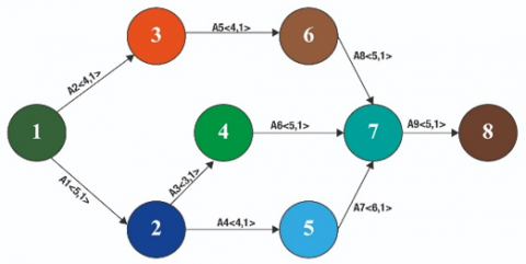
Example 2: Consider the following project networking problem involving interval numbers discussed by Sireesha and Shankar [14] given in Table 3.
Table 3. Activity interval duration of each operation
|
Activity |
Interval time |
|
(A1) 1-2 |
[4,6] |
|
(A2) 1-3 |
[3,5] |
|
(A3) 2-4 |
[2,4] |
|
(A4) 2-5 |
[3,5] |
|
(A5) 3-6 |
[3,5] |
|
(A6) 4-7 |
[4,6] |
|
(A7) 5-7 |
[5,7] |
|
(A8) 6-7 |
[4,6] |
|
(A9) 7-8 |
[4,6] |
Expressing the interval time duration of all the activities in terms of their midpoint width form, the network diagram represented in Figure 7.
By applying the proposed algorithm, the interval critical path of the interval project network is obtained as 1- 2 – 5 – 7 – 8.
The interval completion time of this interval project network is <5,1> + <4,1> + <6,1> + <5,1> = <20,1> = [19,21].
The computational procedure for obtaining earliest start, latest start, earliest finish, latest finish, and total float time and interval critical path is displayed in Table 4. Figure 8 represents the critical path.
Table 4. Computation results of interval earliest and interval latest times
|
Activity |
Interval time |
$\langle m(\tilde{a}), w(\tilde{a})\rangle$ |
Earliest time (Start) |
Earliest time (Finish) |
Latest time (Start) |
Latest time (Finish) |
Total float |
|
(A1) 1-2 |
[4,6] |
<5,1> |
<0,0> |
<5,1> |
<0,0> |
<5,1> |
<0,1> |
|
(A2) 1-3 |
[3,5] |
<4,1> |
<0,0> |
<4,1> |
<2,1> |
<6,1> |
<2,1> |
|
(A3) 2-4 |
[2,4] |
<3,1> |
<5 ,1> |
<8,1> |
<7,1> |
<10,1> |
<2,1> |
|
(A4) 2-5 |
[3,5] |
<4,1> |
<5,1> |
<9,1> |
<5,1> |
<9,1> |
<0,1> |
|
(A5) 3-6 |
[3,5] |
<4,1> |
<4,1> |
<8,1> |
<6,1> |
<10,1> |
<2,1> |
|
(A6) 4-7 |
[4,6] |
<5,1> |
<8,1> |
<13,1> |
<10,1> |
<15,1> |
<2,1> |
|
(A7) 5-7 |
[5,7] |
<6,1> |
<9,1> |
<15,1> |
<9,1> |
<15,1> |
<0,1> |
|
(A8) 6-7 |
[4,6] |
<5,1> |
<8,1> |
<13,1> |
<10,1> |
<15,1> |
<2,1> |
|
(A9) 7-8 |
[4,6] |
<5,1> |
<15,1> |
<20,1> |
<15,1> |
<20,1> |
<0,1> |
Figure 7. Interval project network
Figure 8. Rooted tree representaion of all possible interval paths in the interval project network (Example: 2)
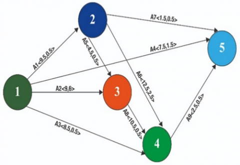
Example 3: Consider the following project networking problem involving interval numbers discussed by Sireesha and Shankar [14] given in Table 5.
Table 5. Activity interval duration of each operation
|
Activity |
Interval time |
|
(A1) 1-2 |
[9,10] |
|
(A2) 1-3 |
[3,15] |
|
(A3) 1-4 |
[8,9] |
|
(A4) 1-5 |
[6,9] |
|
(A5) 2-3 |
[4,5] |
|
(A6) 2-4 |
[10,15] |
|
(A7) 2-5 |
[1,2] |
|
(A8) 3-4 |
[10,11] |
|
(A9) 4-5 |
[2,3] |
Expressing the interval time duration of all the activities in terms of their midpoint width form, the network diagram represented in Figure 9.
By applying the proposed algorithm, the interval critical path of the interval project network is obtained as 1- 2 – 3 – 4 – 5.
The interval completion time of this interval project network is <9.5, 0.5>+<4.5, 0.5>+<10.5, 0.5>+<2.5, 0.5>=<27, 0.5>=[26.5, 27.5].
The computational procedure for obtaining earliest start, latest start, earliest finish, latest finish, and total float time and interval critical path is displayed in Table 6. Figure 10 represent the critical path.
Table 6. Computation results of interval earliest and interval latest times
|
Activity |
Interval time |
$\langle m(\tilde{a}), w(\tilde{a})\rangle$ |
Earliest time (Start) |
Earliest time (Finish) |
Latest time (Start) |
Latest time (Finish) |
Total float |
|
(A1) 1-2 |
[9,10] |
<9.5,0.5> |
<0,0> |
<9.5,0.5> |
<0,0.5> |
<9.5,0.5> |
<0,0.5> |
|
(A2) 1-3 |
[3,15] |
<9,6> |
<0,0> |
<9,6> |
<5,6> |
<14,0.5> |
<5,6> |
|
(A3) 1-4 |
[8,9] |
<8.5,0.5> |
<0,0> |
<8.5,0.5> |
<16,0.5> |
<24.5,0.5> |
<16,0.5> |
|
(A4) 1-5 |
[6,9] |
<7.5,1.5> |
<0,0> |
<7.5,0.5> |
<19.5,1.5> |
<27,0.5> |
<19.5,1.5> |
|
(A5) 2-3 |
[4,5] |
<4.5,0.5> |
<9.5,0.5> |
<14.0.5> |
<9.5,0.5> |
<14,0.5> |
<0,0.5> |
|
(A6) 2-4 |
[10,15] |
<12.5,2.5> |
<9.5, 0.5> |
<22,2.5> |
<12,2.5> |
<24.5,0.5> |
<2.5,2.5> |
|
(A7) 2-5 |
[1,2] |
<1.5,0.5> |
<9.5, 0.5> |
<11,0.5> |
<25.5,0.5> |
<27,0.5> |
<16,0.5> |
|
(A8) 3-4 |
[10,11] |
<10.5,0.5> |
<14,0.5> |
<24.5,0.5> |
<14,0.5> |
<24.5,0.5> |
<0.0.5> |
|
(A9) 4-5 |
[2,3] |
<2.5,0.5> |
<24.5,0.5> |
<27,0.5> |
<24.5,0.5> |
<27,0.5> |
<0,0.5> |
Figure 9. Interval project network
Figure 10. Rooted tree representaion of all possible interval paths in the interval project network (Example: 3)
4.1 Results and discission
The solutions obtained by applying the proposed method are compared with the solutions by other methods in Table 7. It can be seen that the propoed method provides vagueness reduced inervals times in all the cases.
Core benefits of the proposed approach
(1) An alternative way of finding and presenting CPM interval estimates, the most recent hours and slower days are given using intervals as operating time.
(2) The suggested approach reduces the difficulty of model generation and the problem is solved through computation.
(3) Some of the current techniques typically have only smooth solutions for CPM interval problems. We suggest in this paper a straightforward method to discuss the ideal interval treatment of CPM problems and the results obtained without transforming them into classic CPM issues.
Table 7. Comparison of solutions
|
S. No |
Authors |
Critical path time |
Our proposed method |
|
1 |
Shankar and Saradhi [38] |
[100, 260] |
[120,240] |
|
2 |
Sireesha and Shankar [14] |
[16, 24] |
[19,21] |
|
3 |
Sireesha and Shankar [14] |
[25, 29] |
[26.5,27.5] |
While the critical approach to the path is widely criticized today, its history continues to be popular among project managers. CPM has many benefits such as:
The decision maker can pass less critical tasks using CPM, and concentrate his/her attention on maximizing his/her job.
The critical path for the interval project network is 1- 2-3 -5 as shown Figure 6.
The interval completion time of this interval project network is <15, 5>+<45, 15>+<120, 60>=<180, 60>=[120,240].
The critical path for the interval project network is 1- 2 – 5 – 7 – 8 as shown Figure 8.
The interval completion time of this interval project network is <5,1> + <4,1> + <6,1> + <5,1> = <20,1> = [19,21].
The critical path for the interval project network is 1- 2 – 3 – 4 – 5 as shown Figure 10.
The interval completion time of this interval project network is <9.5, 0.5> <4.5, 0.5>+<10.5, 0.5>+<2.5, 0.5>= <27, 0.5>=[26.5, 27.5].
In this paper, we have proposed a new approach for computing the interval time duration of a project networking problems without transforming to crisp equivalent forms. This can be inferred, on the basis of the study results:
In a given project interval network as operating times, a modern way of operating was suggested to find the existing intervals and float times of operations. To get the paths from root to bottom, the network flowchart is described as a rooted tree. New approach to time interval was used to obtain maximum float of any operation. Every action plays a major part in project management as a complete float. Current operator on intervals for finding the most recent interval times is specified. This explained the benefits of the new approach as compared to the current one.
[1] Zadeh, L.A. (1965). Fuzzy sets. Information and Control, 8(3): 338-353. https://doi.org/10.1016/S0019-9958(65)90241-X
[2] Gazdik, I. (1983). Fuzzy-network planning-FNET. IEEE Transactions on Reliability, 32(3): 304-313. https://doi.org/10.1109/TR.1983.5221657
[3] Kaufmann, A., Gupta, M.M. (1988). Fuzzy mathematical models in engineering and management science. Elsevier Science Inc.
[4] McCahon, C.S., Lee, E.S. (1988). Project network analysis with fuzzy activity times. Computers & Mathematics with Applications, 15(10): 829-838. https://doi.org/10.1016/0898-1221(88)90120-4
[5] Hapke, M., Slowinski, R. (1996). Fuzzy priority heuristics for project scheduling. Fuzzy Sets and Systems, 83(3): 291-299. https://doi.org/10.1016/0165-0114(95)00338-X
[6] Yao, J.S., Lin, F.T. (2000). Fuzzy critical path method based on signed distance ranking of fuzzy numbers. IEEE Transactions on Systems, Man, and Cybernetics-Part A: Systems and Humans, 30(1): 76-82. https://doi.org/10.1109/3468.823483
[7] Slyeptsov, A.I., Tyshchuk, T.A. (2003). Fuzzy temporal characteristics of operations for project management on the network models basis. European Journal of Operational Research, 147(2): 253-265. https://doi.org/10.1016/S0377-2217(02)00559-3
[8] Dubois, D., Fargier, H., Galvagnon, V. (2003). On latest starting times and floats in activity networks with ill-known durations. European Journal of Operational Research, 147(2): 266-280. https://doi.org/10.1016/S0377-2217(02)00560-X
[9] Chen, S.P. (2007). Analysis of critical paths in a project network with fuzzy activity times. European Journal of Operational Research, 183(1): 442-459. https://doi.org/10.1016/j.ejor.2006.06.053
[10] Chen, C.T., Huang, S.F. (2007). Applying fuzzy method for measuring criticality in project network. Information Sciences, 177(12): 2448-2458. https://doi.org/10.1016/j.ins.2007.01.035
[11] Chen, S.P., Hsueh, Y.J. (2008). A simple approach to fuzzy critical path analysis in project networks. Applied Mathematical Modelling, 32(7): 1289-1297. https://doi.org/10.1016/j.apm.2007.04.009
[12] Cheng, F., Lin, M., Yüksel, S., Dinçer, H., Kalkavan, H. (2020). A hybrid hesitant 2-tuple IVSF decision making approach to analyze PERT-based critical paths of new service development process for renewable energy investment projects. IEEE Access, 9: 3947-3969. https://doi.org/10.1109/ACCESS.2020.3048016
[13] Sireesha, V., Shankar, N.R. (2010). A new approach to find total float time and critical path in a fuzzy project network. International Journal of Engineering Science and Technology, 2(4): 600-609.
[14] Sireesha, V., Rao, K.S., Shankar, N.R., Babu, S.S. (2012). Critical path analysis in the network with fuzzy interval numbers as activity times. International Journal of Engineering Science and Technology (IJEST), 4(3): 823-832.
[15] Mukherjee, S., Basu, K. (2011). Solution of interval PERT/CPM network problems by a simplified tabular method. Opsearch, 48: 355-370. https://doi.org/10.1007/s12597-011-0056-z
[16] Shanmugasundari, M., Ganesan, K. (2014). Project scheduling problems under fuzzy environment: A new solution approach. International Journal of Pure and Applied Mathematics, 95(3): 387-399. http://dx.doi.org/10.12732/ijpam.v95i3.6
[17] Zhu, J., Huang, G. (2016). An interval parameter two-stage stochastic approach to optimize budget and schedule in construction management. Journal of Civil & Environmental Engineering, 6(3): 1-9. http://dx.doi.org/10.4172/2165-784X.1000228
[18] Yogashanthi, T., Ganesan, K. (2017). Modified critical path method to solve networking problems under an intuitionistic fuzzy environment. ARPN Journal of Engineering and Applied Sciences, 12(2): 398-403.
[19] Mohagheghi, V., Mousavi, S.M., Vahdani, B. (2017). An assessment method for project cash flow under interval-valued fuzzy environment. Journal of Optimization in Industrial Engineering, 10(22): 73-80.
[20] Prater, J., Kirytopoulos, K., Ma, T. (2017). Optimism bias within the project management context: A systematic quantitative literature review. International Journal of Managing Projects in Business, 10(2): 370-385. https://doi.org/10.1108/IJMPB-07-2016-0063
[21] Ibadov, N. (2019). Construction project planning under fuzzy time constraint. International Journal of Environmental Science and Technology, 16(9): 4999-5006. https://doi.org/10.1007/s13762-018-1695-x
[22] Kholil, M., Alfa, B.N., Hariadi, M. (2018). Scheduling of house development projects with CPM and PERT method for time efficiency (Case study: House type 36). In IOP Conference Series: Earth and Environmental Science, 140(1): 012010. https://doi.org/10.1088/1755-1315/140/1/012010
[23] Mahmoud, A.H. (2019). Critical paths in a fuzzy Construction project network. International Journal of Civil Engineering and Technology (IJCIET), 10(1): 1313-1321.
[24] Begum, S.G., Praveena, J.P.N., Rajkumar, A. (2019). Critical path through interval valued hexagonal fuzzy number. International Journal of Innovative Technology and Exploring Engineering, 8(11): 1190-1193.
[25] Raju, V., Paruvatha Vathana, M. (2019). Fuzzy critical path method with icosagonal fuzzy numbers using ranking method. JAC: A Journal of Composition Theory, VII(IX), 62-69.
[26] Senouci, A., Leon, R.M., Eldin, N. (2019). Schedule performance index effectiveness in assessing project schedule performance. International Journal of Construction Engineering and Management, 8(2): 46-55. https://doi.org/10.5923/j.ijcem.20190802.02
[27] Dorfeshan, Y., Mousavi, S.M., Vahdani, B., Siadat, A. (2018). Determining project characteristics and critical path by a new approach based on modified NWRT method and risk assessment under an interval type-2 fuzzy environment. Scientia Iranica, 26(4): 2579-2600. https://dx.doi.org/10.24200/sci.2018.50091.1503
[28] Ramesh, G., Sudha, G., Ganesan, K. (2019). A study on interval PERT/CPM network problems. In AIP Conference Proceedings, 2112(1): 020123. https://doi.org/10.1063/1.5112308
[29] Rameshan, N., Dinagar, D.S. (2020). Solving fuzzy critical path with octagonal intuitionistic fuzzy number. In AIP Conference Proceedings, 2277(1): 090002. https://doi.org/10.1063/5.0025360
[30] Rameshan, N., Dinagar, D.S. (2022). A study on fuzzy critical path with quadrilateral fuzzy numbers. Advances and Applications in Mathematical Sciences, 21(3).
[31] Ganesh, A.H., Shobana, A.H. (2020). On optimizing interval data based critical path problem for the analysis of various fuzzy quantities using fuzzification and centroid based defuzzification techniques. Malaya Journal of Matematik, S(1): 319-330. https://doi.org/10.26637/MJM0S20/0060
[32] Liu, D., Hu, C. (2021). A dynamic critical path method for project scheduling based on a generalised fuzzy similarity. Journal of the Operational Research Society, 72(2): 458-470. https://doi.org/10.1080/01605682.2019.1671150
[33] Mirnezami, S.A., Mousavi, S.M., Mohagheghi, V. (2021). An innovative interval type-2 fuzzy approach for multi-scenario multi-project cash flow evaluation considering TODIM and critical chain with an application to energy sector. Neural Computing and Applications, 33: 2263-2284. https://doi.org/10.1007/s00521-020-05095-z
[34] Karthy, T., Sandhya, P. (2022). Fuzzy critical path analysis. AIP Conference Proceedings, 2516: 200030. https://doi.org/10.1063/5.0108690
[35] Shankar, N.R., Sireesha, V., Rao, P.P.B. (2010). An analytical method for finding critical path in a fuzzy project network. International Journal of contemporary Mathematical Sciences, 5(20): 953-962.
[36] Sengupta, A., Pal, T.K. (2000). On comparing interval numbers. European Journal of Operational Research, 127(1): 28-43. https://doi.org/10.1016/S0377-2217(99)00319-7
[37] Ma, M., Friedman, M., Kandel, A. (1999). A new fuzzy arithmetic. Fuzzy Sets and Systems, 108(1): 83-90. https://doi.org/10.1016/S0165-0114(97)00310-2
[38] Shankar, N.R., Saradhi, B.P. (2011). Fuzzy critical path method in interval-valued activity networks. International Journal of Pure and Applied Sciences and Technology, 3(2): 72-79.