Abhishek Kumar*![]() | Om Prakash
| Om Prakash![]()
© 2023 IIETA. This article is published by IIETA and is licensed under the CC BY 4.0 license (http://creativecommons.org/licenses/by/4.0/).
OPEN ACCESS
The paper deals with the nonlinear mathematical modelling of the longitudinal dynamics of a small sized hybrid airship with suspended payload vehicle. The modelling is done by considering the system as single body dynamic as well as two body dynamics. Bifurcation Analysis method is applied to do the trim and stability analysis of the system. MATLAB and AUTO bifurcation analysis tool is used for dynamic modeling and simulation of the system. Total five different simulation cases with different elevator deflection are discussed for 3DOF model. For each case Six output states as Vel, gamma, alpha, q, theta and range (h) is taken and one input parameter as dele i.e. elevator deflection is taken. In this paper 6DOF and 3DOF longitudinal conventional single body dynamic model of hybrid airship is discussed and an alternate method as 4DOF two body longitudinal dynamic model of hybrid airship is also considered. Simulation is done for all models on MATLAB and Alternate technique as bifurcation method is also used on AUTO software to study the dynamic analysis of the system. Eigen values is obtained from bifurcation method and is helpful to analyze the stability of the Hybrid airship with suspended payload vehicle.
bifurcation analysis, dynamic simulation, hybrid airship with suspended payload, stability, trim analysis, 3DOF and 4 DOF longitudinal
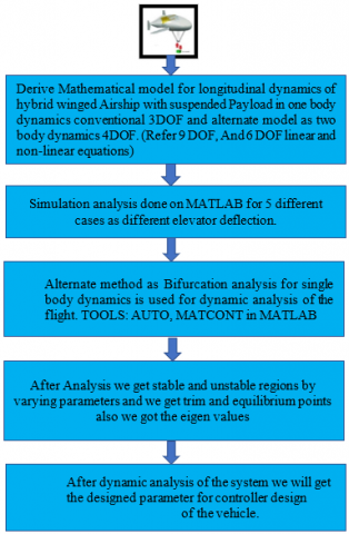
A conventional airship design consists of an axisymmetric, teardrop-shape hull filled with lifting gas, a pair of horizontal and vertical tail fins for providing weathercock stability and control, a propulsion system for thrust power, and a gondola for carrying payloads. The common lifting gasses that are used in the airship are hydrogen and helium. An airship cruises at a very low speed, with an average airspeed of 20m/s [1], thus its flying and handling performance is significantly affected by the wind. When in trim flight and on the ground, the airship must always maintain nearly neutral buoyancy for stability, so the airship’s weight and trim setting must be adjusted constantly when in flight. Because of the promising and favourable qualities of the airship, such as its hovering ability, extended endurance, heavy lifting and low energy consumption, the interest in hybrid airship design has been increasing recently. Hybrid airship includes the features of the vehicle which is lighter than air and the vehicle which is heavier than air. It generates a fraction of its total lift from buoyancy, while the remainder of the lift is generated aerodynamically and through the propulsion system [2]. With the aid of its static buoyant lift and the wing's contribution to the airship's stability and control, the hybrid winged airship is theoretically able to sustain prolonged flight duration. The integrated wing on the hull also provides the airship a safer means to descent to the ground in the case of failures such as a loss of helium in flight, where the airship is able to control its manoeuvrability from the wing, and in the case of engine failure, the airship is able to glide while still having a certain degree of manoeuvrability control. The hybrid winged airship, if designed properly, can fulfil the demanding requirement of a low-speed air vehicle with high endurance and satisfactory controllability, which gives it the capability of hovering or loitering in space for an extended amount of time. If the hybrid winged airship is designed to be remotely operated, its endurance is only limited by the propulsion system, but solar panel can be opted in the design for longer endurance. Overall, this hybrid airship design provides a feasible and economical solution for aerial surveillance application. Coming up with a mathematical model at the preliminary stage of development is difficult due to the lack of insight of the hybrid airship’s characteristic and behaviour. But there are estimation methods that can be used for some values of the parameters involved in the mathematical model. To help with the derivation of the mathematical model, all important preliminary sizing and weight estimation will be carried out. Although the hybrid airship is unique, its modelling and stability analysis were done according to the typical procedure of a conventional airship and aircraft. Analysis of parafoil system using trim and stability from researches [3-5] uses bifurcation technique and discusses the impact of the model constraints on the longitudinal dynamics with trim along with stability traits for 4DOF longitudinal dynamic flight model. 4DOF comes from 9DOF model of hybrid airship discussed in researches [6-7]. Analysis of trim conditions [8-10] for nonlinear flight control law development is carried out using a model-based control structure. It shows trimmed flight analysis using outer loop and inner loop equations in the 6DOF aircraft model for different control surface deflections. Trim analysis using equations of motion for aircraft design is presented for steady-state straight flight [11, 12] and for turning, pull up and pull overflight [12]. Hybrid-Airships exist in different configurations [13-16]. The study is related to trimming the 6DOF conventional and unconventional aircraft for control power assessment and to formulate a generic analytical framework for trim analysis. The longitudinal flight dynamics play a vital role in the flight manoeuvres as most of the flight duration corresponds to longitudinal flight dynamics in the longitudinal frame. Longitudinal flight includes the complete flight regime, comprising velocity in the fixed X and Z plane of the body, and level flight, climb and descent, and pull-up and pull-down flight. This shows that longitudinal flight dynamics should be the major concern for the trim and stability analysis. This paper provides the trim analysis of the small sized of hybrid airship's longitudinal dynamic model and its stability analysis. It provides the trim simulation of the hybrid airship for the complete flight envelope for elevator deflection from dele =-15 to 15 degrees, and its dynamic analysis using the Bifurcation Method considering the eigenvalues approach and longitudinal modes analysis of the hybrid airship flight in one body dynamics and two body dynamics approach. The research methodology is shown below in Figure 1.
Figure 1. Methodology flow chart
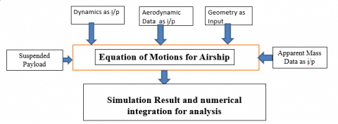
The proposed model, a winged hybrid small-sized airship flight vehicle with a suspended payload, appears in Figure 2 and will be used for modelling and analysis in this research. A winged aircraft, an airship, and aircraft elements known as the Plimp and parafoil payload delivery flight system was combined to make the model, which is in the first row and first column. Figure 3 depicts the workflow for creating airship nonlinear flight dynamics models and simulations. The associated payload is assumed to be carried by the hybrid airship.
Figure 2. Winged hybrid airship flight vehicle design concept with suspended payload [17]
Figure 3. Flow chart for mathematical modelling [17]
Table 1. Complexity chart in mathematical derivation
|
Mathematical modelling terms |
Aircraft |
Parafoil system (parachute/Glider) |
Hybrid airship |
|
Apparent mass |
NO |
YES |
YES |
|
Buoyancy |
NO |
YES |
YES |
|
Aerodynamic data |
YES |
YES |
YES |
|
Geometric data |
YES, without apparent mass |
YES, with apparent mass |
YES, with apparent mass |
|
Aerodynamics |
YES |
YES |
YES |
|
Flight dynamics |
EOM is at CG |
EOM is at CG |
EOM is at CV |
In comparison to an aircraft or a parafoil delivery mode, the mathematical modelling of a hybrid airship with payload is more challenging, as it indicates in the above Table 1. Due to the fact that the centres of mass or gravity and volume are situated at two different locations, as indicated in Figure 4, the mathematical derivation of a hybrid airship is challenging. At the centre of mass or centre of gravity, it is simple to obtain the moment equation and force equation. In a hybrid airship, the centre of volume is almost exactly in the middle of the hull, which is filled with helium or hydrogen gas. In a hybrid airship, the payload's attached gondola is close to the centre of mass, or centre of gravity.
Figure 4. Coordinate location of CG and CV [18]
2.1 3-DOF single body dynamic longitudinal model
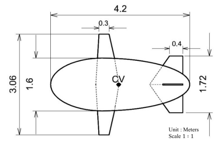
A Hybrid Airship is modelled and simulated using assumptions as the flat Earth approximation, airship considered as rigid body, mass and volume of hybrid airship assumed as constant, centre of volume and centre of buoyancy is assumed to coincide, and atmosphere is assumed as stationary. For study or analysis purpose international atmospheric conditions are followed for flight dynamic analysis. The whole volume of airship under study is usually filled with lighter than air helium gas, that’s why centre of buoyancy is assumed to coincide with centre of volume. Equations of motion are established using Newton's and Euler's equations for general aircraft in addition of the added mass and inertia effects and buoyancy force. The geometric specifications and data of the vehicle is given in Tables 2 and 3.
Table 2. Geometry data of a HULL [18]
|
Parameter of a HULL |
Value |
|
Mass of a Hull, mh |
10 kg |
|
Overall Airship length, l |
3.75 m |
|
Maximum Airship Diameter, D |
1.6 m |
|
Hull Volume, V |
5.6 m3 |
|
Reference Area of a Hull, Sk |
3.16 m2 |
|
Reference length of a Hull, c |
1.78 m |
|
Ellipsoid shaped semi-minor axis, b |
0.8 m |
|
Airship Wingspan, b |
3.06 m |
|
Airship Wing area, S |
1.72 m2 |
|
Airship tail span, bt |
3.06 m |
|
Airship tail area, St |
0.916 m2 |
|
Rck |
0.8 m |
Table 3. Payload geometry [18]
|
Parameter of payload |
Value |
|
mb |
2 kg |
|
Sb |
0.1x0.2 m2 |
|
Rcb |
0.25 m |
|
C DB |
1.05 |
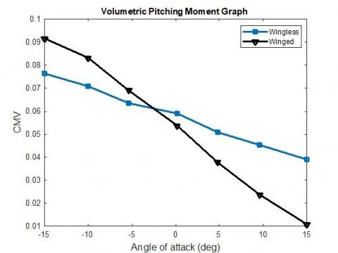
The geometric view of the vehicle with specifications is shown in Figure 5. Figure 6 shows the aerodynamic data plot of airship taken from researches [2, 18].
The complete Non-linear 6 DOF equation of motion of a Hybrid airship is given in Eq. (1).
$\left\lceil\begin{array}{cc}m I_3+M^{\prime} & -m r_G^X \\ m r_G^X & I_0+I_0^{\prime}\end{array}\right]\left[\begin{array}{c}\dot{V}_0 \\ \dot{\omega}_0\end{array}\right]+\left[\begin{array}{c}m\left(\omega_0 \times V_0+\omega_0 \times\left(\omega_0 \times r_G\right)\right) \\ \omega_0 \times\left(I_0 \omega_0\right)+m r_G \times\left(\omega_0 \times V_0\right)\end{array}\right]=\left[\begin{array}{l}F \\ \zeta\end{array}\right]$ (1)
where,
$r_G^X=\left[\begin{array}{ccc}0 & -a_z & a_y \\ a_z & 0 & -a_x \\ -a_y & a_x & 0\end{array}\right]$ (2)
$\left(r_G^X\right)^T=-\left(r_G^X\right)$ (3)
The complete Non-linear 6 DOF equation of motion for an Aircraft [19] is given in Eq. (4).
$\left[\begin{array}{cc}m I_3 & 0 \\ 0 & I_0\end{array}\right]\left[\begin{array}{l}\dot{V}_0 \\ \dot{\omega}_0\end{array}\right]+\left[\begin{array}{c}m\left(\omega_0 \times V_0\right) \\ \omega_0 \times\left(I_0 \omega_0\right)\end{array}\right]=\left[\begin{array}{l}F \\ \zeta\end{array}\right]$ (4)
Figure 5. Top view of winged hybrid airship [18]
(a) CLV vs $\alpha$
(b) CDV vs $\alpha$
(c) CMV vs $\alpha$
Figure 6. Aerodynamic data [2, 18]
Figure 7. Flowchart for apparent mass calculation for hybrid airship
Addition of the apparent mass calculation in hybrid airship is shown in Figure 7. The hybrid airship is lighter than air vehicle and it consists of HULL filled with hydrogen/helium gas. So, apparent mass calculation, buoyancy force equation and mass distribution are important in the mathematical modelling of a hybrid airship. Contribution of mass components in hybrid airship is shown in Figure 8.
Figure 8. Mass distribution
The volume for hydrostatic lift provided in Eq. (5) and the Archimedes principle were used to calculate the lift in airship design (6).
$L_{h s t}=\operatorname{vol}\left(\rho_a-\rho_a\right)$ (5)
where, ρa and ρg are the densities of air and lifting gas.
$w_{\text {net }}=\left(m_{\text {GTw }} \times g-L_{\text {hst }}\right)$ (6)
The weight balanced by the hydrostatic lift is subtracted from the gross take-off weight to get the net weight, or wnet. The equation for the hybrid airship's propulsion system is given as Eq. (7a) to (7c).
$M_P=M_T=T d_z$ (7a)
$X_P=X_T=T$ (7b)
$Z_P=Z_T=0$ (7c)
T is the total thrust produced by the engine, MT is the moment owing to the propulsion system or thrust, and dz is the distance between the propulsion system and the CV. The full nonlinear forces and moments equation for the 3DOF longitudinal dynamics is given in Eq. (8) to (11), which includes the axial force equation (U), normal force equation (W), pitching moment equation (q), and kinematic equation (θ ̇).Where Xa is axial aerodynamic force, XS is axial buoyancy force, XT is axial thrust force, Za is normal aerodynamic force, ZS is buoyancy force in normal direction along z-axis, ZT is normal thrust force, Ma is aerodynamic pitching moment along y-axis, Ms is buoyancy pitching moment due to buoyancy about CG and MT is thrust moment along y-axis or pitching moment.
2.1.1 Non-linear longitudinal dynamic equations for hybrid airship
Force equations:
Axial force:
$m_x \dot{U}+\left(m a_x-X_{\dot{q}}\right) \dot{q}+m_z q W-m a_x q^2=X_a+X_S+X_T$ (8)
Normal force:
$m_z \dot{W}-\left(m a_x+Z_{\dot{q}}\right) \dot{q}-m_x q U+m a_z q^2=Z_a+Z_S+Z_T$ (9)
Moment equations:
Pitching moment:
$J_y \dot{q}+\left(m a_z+M_{\dot{u}}\right) \dot{U}-\left(m a_x+M_{\dot{w}}\right) \dot{W}+m a_x(q U)+m a_z(q W)=M_a+M_s+M_T$ (10)
Kinematic equation:
$\dot{\theta}=q$ (11)
In linearizing the nonlinear equation of motion from Eqns. (8) to (11), small perturbation theory is applied, where squares of variables and coupling derivatives are omitted and small angle assumption is used. An example of a complete expression of the aerodynamic force in x-axis is given in Eq. (12).
$X_a=X_1+X_u \cdot u+X_v \cdot v+X_w \cdot w+X_p \cdot p+X_q \cdot q+X_r \cdot r$ (12)
where, X1 is the trim equilibrium aerodynamic force which is defined as:
$X_1=\frac{1}{2} \rho_{a i r} V^2 s\left(C_L \sin \alpha-C_D \cos \alpha\right)$ (13)
The rest of the components in the aerodynamic expression are the dynamic perturbations terms, which will be zero if the aircraft is in equilibrium. Some of the terms in the aerodynamic force and moment representation can be neglected if its contribution to the motion is very small [20, 21].
2.1.2 Linearized longitudinal dynamic equations for hybrid airship
Force equations:
Axial force:
$m_x \dot{U}+\left(m a_x-X_{\dot{q}}\right) \dot{q}+m_z q W_1=X_a+X_S+X_T$ (14)
Normal force:
$m_z \dot{W}-\left(m a_x+Z_{\dot{q}}\right) \dot{q}-m_x q U_1=Z_a+Z_S+Z_T$ (15)
Moment equations:
Pitching moment:
$J_y \dot{q}+\left(m a_z+M_{\dot{u}}\right) \dot{U}-\left(m a_x+M_{\dot{w}}\right) \dot{W}+m a_x(q U)+m a_z(q W)=M_a+M_s+M_T$ (16)
Kinematic equation:
$\dot{\theta}=q$ (17)
The expression of the aerodynamic force in x-axis shown in Eq. (12) is expressed below for longitudinal dynamics of the Airship.
$X_a=X_1+X_u \cdot u+X_w \cdot w+X_q \cdot q+X_{\delta_e} \cdot \delta_e$ (18)
Table 4. Longitudinal stability derivatives
|
u derivatives |
w derivatives |
|
$X_u=\frac{-2 C_{D_1} q_1 S}{U_1}$ |
$X_w=\frac{-\left(C_{D_\alpha}-C_{L_1}\right) q_1 S}{U_1}$ |
|
$Z_u=\frac{-2 C_{L_1} q_1 S}{U_1}$ |
$Z_w=\frac{-\left(C_{L_\alpha}+C_{D_1}\right) q_1 S}{U_1}$ |
|
$M_u=\frac{C_{m_1 q_1 S \bar{c}}}{U_1}$ |
$M_w=\frac{C_{m_\alpha} q_1 s \bar{c}}{U_1}$ |
|
q derivatives |
$\delta_e$ derivatives |
|
$X_q=\frac{-C_{D_q q_1 S \bar{c}}}{2 U_1}$ |
$X_{\delta_e}=\frac{-C_{D_{\delta_e}} q_1 S \bar{c}}{2 U_1}$ |
|
$Z_q=\frac{-C_{L_q} q_1 S \bar{c}}{2 U_1}$ |
$Z_{\delta_e}=\frac{-C_{L_{\delta_e}} q_1 S \bar{c}}{2 U_1}$ |
|
$M_q=\frac{C_{m_q} q_1 S \bar{c}^{\mathbf{2}}}{2 U_1}$ |
$M_{\delta_e}=\frac{C_{m_{\delta_e}} q_1 S \bar{c}^2}{2 U_1}$ |
The expression for the stability derivatives is given in the Table 4. The aerodynamic coefficients (such as, $C_{m_\alpha}, C_{m_q}$ and $c_{m_{\delta_e}}$) are obtained either from wind tunnel test, numerical solutions, or semi-empirical approach [18-22]. For a complete analysis, the aerodynamic database that includes all the expression of the aerodynamic coefficients must be constructed for the vehicle. Since the hybrid airship is newly developed, such database has not been created. The main challenge here is that there is no source in the open literature that tackles the problem of estimating the aerodynamic coefficients of a winged hybrid airship, while there are several approximation methods for conventional aircrafts [23, 24]. With the assumption that the general equation for an aircraft is adequate for the winged airship application as well, the remaining aerodynamic coefficients are estimated using estimation methods and equations provided by studies [25, 26]. The estimates are only sufficient for this preliminary modelling and analysis of the winged hybrid airship. To ensure the accuracy of these aerodynamic coefficients, CFD and wind tunnel test must be performed on a model of the hybrid airship.
2.1.3 Buoyancy or static forces and moments:
The buoyancy forces and moments for hybrid airship is given in Eq. (19a) to (19c).
$X_s=-(m g-B) \sin \theta$ (19a)
$Z_s=(m g-B) \cos \phi \cos \theta$ (19b)
$M_s=-\left(m g a_z+B b_z\right) \sin \theta-\left(m g a_x+B b_x\right) \cos \phi \cos \theta$ (19c)
3DOF hybrid airship Longitudinal translational and rotational dynamics Eqns. (8-11) of the model can be transformed and modelled into the Eqns. (37-44) using the wind axis representation and are given by:
$\dot{\mathrm{V}}=\left(\mathrm{T} \cos (\alpha)-\overline{\mathrm{q}} \mathrm{sC}_{\mathrm{D}}-(\mathrm{mg}-\mathrm{B}) \sin (\gamma)\right) /\left(\mathrm{m}-\mathrm{X}_{\mathrm{ud}}\right)$ (20)
$\dot{\gamma}=\left(T \sin (\alpha)+\overline{\mathrm{q}}_{\mathrm{S}} C_\mathrm{L}+\mathrm{z}_{\mathrm{q}}-(m g-B) \cos (\gamma)\right) /\left\{\left(\mathrm{m}-\mathrm{z}_{\mathrm{wd}}\right) \cdot \mathrm{V}\right\}$ (21)
$\dot{\mathrm{q}}=\mathrm{M}_{\mathrm{z}} /\left(\mathrm{I}_{\mathrm{yy}}-\mathrm{Mq}_{\mathrm{d}}\right)$ (22)
$\dot{\theta}=q$ (23)
$\dot{R}=V \cos (\gamma)$ (24)
$\dot{h}=V \sin (\gamma)$ (25)
Considering α=θ-γ, So:
$\dot{\alpha}=q-\left[\left(T \sin (\alpha)+\overline{\mathrm{q}} s\mathrm{C}_1+\mathrm{z}_{\mathrm{q}}-(m g-B) \cos (\gamma)\right) /\left\{\left(\mathrm{m}-\mathrm{z}_{\mathrm{wd}}\right) \cdot \mathrm{V}\right\}\right.$ (26)
$M_z=-M_s+\left(M q-m a_x u u-m a_z w w\right) \cdot q+\bar{q} S \bar{c} C_{m_{m p}}+T * 0 \cdot 1$ (27)
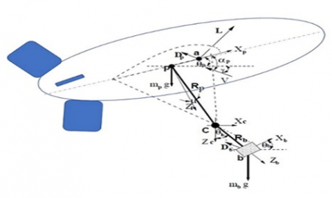
2.2 4-DOF two body dynamic longitudinal model
To achieve the intended goal, a mathematical model of the hybrid airship is created by applying physical principles that describe the hybrid airship's non-linear dynamics and aerodynamics. Combining the 3DOF longitudinal dynamics of the hybrid airship with wing with the 3DOF equation of motion of the suspended payload, the 4DOF model of the hybrid airship with suspended payload has been suggested, as illustrated in Figure 9. A two-body dynamic 4DOF model of a hybrid airship with a hanging payload is presented in the research [17]. Multibody approach discussed in the research [27, 28] also. Thrust is equal to drag force in the airship dynamic model for level flight when the velocity is constant at 20 m/s. The effects of elevator at wing and moment at fin are also considered in the moment equation [17]. An apparent mass is also taken care in the modelling.
Figure 9. Longitudinal 4 DOF Two body dynamics for the hybrid airship payload system [7]
A 4-DOF dynamic model of a hybrid airship with suspended payload developed in the research [7] is shown below.
$\left[\begin{array}{cccccc}m_b \cos \theta_b & -m_b \sin \theta_b & m_b R_b & 0 & \cos \theta_b & -\sin \theta_b \\ m_b \sin \theta_b & m_b \cos \theta_b & 0 & 0 & \sin \theta_b & \cos \theta_b \\ 0 & 0 & I_b & 0 & -R_b \cos \theta_b & R_b \sin \theta_b \\ m_{p A} \cos \theta p & -m_{p A} \sin \theta p & 0 & m_{P A} R p \cos \mu & -\cos \theta_p & \sin \theta_p \\ m_{P C} \sin \theta_P & m_{P C} \cos \theta_P & 0 & -m_{p c} R_P \sin \mu & -\sin \theta_p & -\cos \theta_p \\ 0 & 0 & 0 & I_{P F} & z_{c p} & -x_{C p}\end{array}\right]\left[\begin{array}{c}\dot{u}_c \\ \dot{w}_C \\ \dot{q}_b \\ \dot{q}_p \\ F_x \\ F_z\end{array}\right]=\left\{\begin{array}{l}b_1 \\ b_2 \\ b_3 \\ b_4 \\ b_5 \\ b_6\end{array}\right\}$ (28)
$b_1=-m_b g \sin \theta_b-\mathbb{Q}_b S_b C_{D_b} \cos \alpha_b$ (29a)
$b_2=m_b g \cos \theta_b-Q_b S_b C_{D_b} \sin \alpha_b+m_b R_b q_b^2$ (29b)
$b_3=0$ (29c)
$b_4=-m_p g \sin \theta_p+\mathbb{Q}_p S_p C_x+m_{p c} R_p \sin \mu q_p^2-(C-A)\left(u_C \sin \theta_P+w_C \cos \theta_p\right) q_p$ (29d)
$b_5=m_P g \cos \theta p+Q_p S_\rho C_z+m_{p A} R_p \cos ^\mu q_P^2-(C-A)\left(U_C \cos \theta_P-w_C \sin \theta_p\right) q_p$ (29e)
$b_6=-x_{p a} Q_p S_p C_z+Q_p S_{P C} C_M$ (29f)
2.3 Aerodynamic model and longitudinal trim analysis
MATLAB is used to create subroutines for the model simulation. The lift force, drag force and pitching moment are expressed by L=qSCL, D=qSCDand M=qcSCm and the lift coefficient, drag coefficient and pitching moment coefficient are given by the Eqns. (30-32). These linear relations of aerodynamic coefficients given by Eqns. (30-32) are considered for the 3DOF longitudinal model simulation of hybrid airship and are also used to implement the bifurcation method with the elevator deflection $\delta_e$.
$C_L=\left\{C_{L_0}+C_{L_\alpha} \cdot \alpha+C_{L_q} \cdot \frac{q \bar{c}}{2 V_1}+C_{L_{\delta_e}} \cdot \delta_e\right\}$ (30)
$C_D=\left\{C_{D_0}+C_{D_\alpha} \cdot \alpha+C_{D_q} \cdot \frac{q \bar{c}}{2 V_1}+C_{D_{\delta_e}} \cdot \delta_e\right\}$ (31)
$C_m=\left\{C_{m_0}+C_{m_\alpha} \cdot \alpha+C_{m_q} \cdot \frac{q \bar{c}}{2 V_1}+C_{m_{\delta_e}} \cdot \delta_e\right\}$ (32)
For the static longitudinal stability of the vehicle, the value of Cm must be negative, and the value of positive and negative Cm refer to nose up and nose down pitching moment respectively, Cm changes with the change of α.
The longitudinal nonlinear dynamic hybrid airship model presented with Eqns. (20-27) is used to obtain the solution for the trim or equilibrium state. These states are V, γ, q, θ and α, in which the states V, γ and θ are considered to be zero, i.e., considering the model to be flying with constant V, γ and θ values. In this situation the flight is in a straight path with the possible conditions as γ=0 for the level flight, γ=positive value for the ascend flight or γ=negative value for the descending flight, and at the same time with the constraint that the nose orientation is constant i.e., θ=constant. To achieve these trim conditions for the hybrid airship flight, we obtain the trim states by setting left-hand side of Eqns. (20-27) to zero and solving for the right-hand side, and this is given by Eqns. (33-37).
$0=\left(\mathrm{T} \cos (\alpha)-\overline{\mathrm{q}} s\mathrm{C}_{\mathrm{D}}-(\mathrm{mg}-\mathrm{B}) \sin (\gamma)\right) /\left(\mathrm{m}-\mathrm{X}_{\mathrm{ud}}\right)$ (33)
$0=\left(T \sin (\alpha)+\overline{\mathrm{q}} \mathrm{sC}_{\mathrm{L}}+\mathrm{z}_{\mathrm{q}}-(m g-B) \cos (\gamma)\right) /\left\{\left(\mathrm{m}-\mathrm{z}_{\mathrm{wd}}\right) \cdot \mathrm{V}\right\}$ (34)
$0=\mathrm{M}_{\mathrm{z}} /\left(\mathrm{I}_{\mathrm{yy}}-\mathrm{Mq}_{\mathrm{d}}\right)$ (35)
$\dot{\theta}=0$ (36)
The trim states are represented by (*) and are given by the following Eqns. (37-39).
$C_D^*=(\mathrm{T} \cos (\alpha)-(\mathrm{mg}-\mathrm{B}) \sin (\gamma)) / \bar{q} \mathrm{s}$ (37)
$C_L^*=\left((m g-B) \cos (\gamma)-T \sin (\alpha)-\mathrm{z}_{\mathrm{q}}\right) /\bar{q} \mathrm{s}$ (38)
$C_m^*=\left(M_s-\left(M q-m a_x u u-m a_z w w\right) \cdot q-T * 0 \cdot 1\right) / \bar{q} S c$ (39)
From Eq. (37) we can write the thrust relation given by Eq. (40).
$\mathrm{T}=(\mathrm{mg}-\mathrm{B}) \sin (\gamma)+C_D^* \overline{\mathrm{q}}^* \mathrm{~s} / \cos (\alpha)$ (40)
The initial values for the simulation are also used as the initial values to implement the bifurcation method.
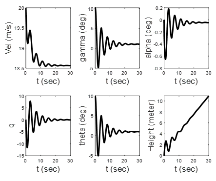
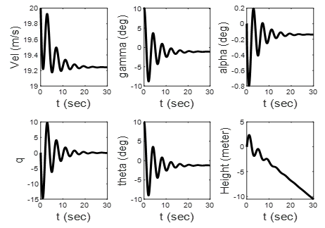
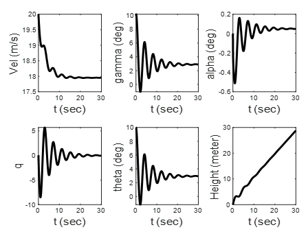
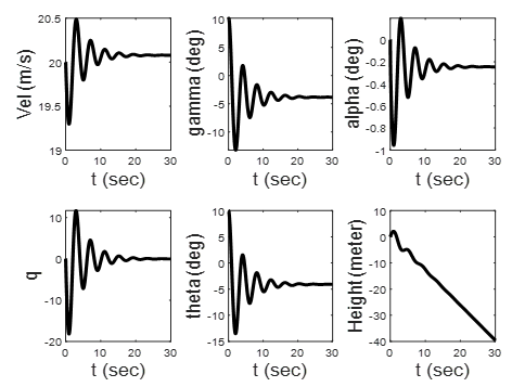
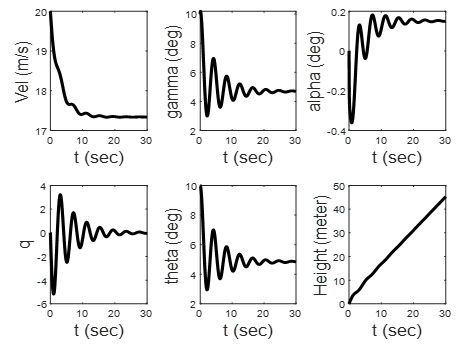
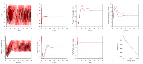
The dynamic stability analysis of the hybrid airship model at different elevator deflection is performed in level flight. Case 1 simulation shown in Figure 10, shows that the angle of attack α, q, theta and gamma is stabilizing 0 degrees with the decrease in the hybrid airship speed for elevator deflection, δe=0 degree, and with the gain in height. The overall dynamic simulation for the case shows the stable short period dynamic behaviour and the angle of attack α shows converging nature, near the equilibrium or trim point. Some more simulation time will show long period dynamic behaviour. Case 2 simulation shown in Figure 11 shows that the angle of attack α, pitch rate q, and theta is stabilizing 0 degrees with the decrease in the hybrid airship speed in oscillatory nature for elevator deflection, δe=-1.5 degree, and with the oscillatory gain in height in opposite direction. The flight path angle gamma maintains the flight of γ=-0.2 degrees and settles after 25 sec. The overall dynamic trim simulation for the case shows a stable behaviour and the angle of attack, α shows a divergence nature, near to the equilibrium or trim point. Case 3 simulation shown in Figure 12, shows that the angle of attack, α is stabilizing near α=-0.22 degrees with the decrease in the hybrid airship speed for elevator deflection, δe=-1.5 degree, and with height gain sharply. The flight path angle, γ increases from γ=0 to 4.6 degrees and the pitch rate, q is stabilized near q=0. Theta stabilizes near 4.36 degree. The overall dynamic simulation for the case shows the stable behaviour and the angle of attack, α shows the convergent nature, near to the equilibrium or trim point. Case 4 simulation shown in Figure 13, shows that the angle of attack, α is stabilizing near α=-0.44 degrees after 25 sec with the airship speed settles at trim value of 19.67 m/s for elevator deflection, δe=3.154 degree, and with height gain in opposite direction. The flight path angle, γ maintains the flight at -2.6 degree and the pitch rate, q is maintained near to q=0. The overall dynamic simulation for the case shows the stable behaviour and the angle of attack, α shows convergent nature, near the equilibrium or trim point. Case 5 simulation shown in Figure 14, shows that the angle of attack, α settles near α=-0.15 degrees with the breaking down the airship speed at 17.26 m/s after 15 sec for elevator deflection, δe=-3.154 degree, and with the gain in altitude in positive direction. The flight path angle, γ maintains the flight of γ=6.5 degrees and the pitch rate, q also settles down to 0 with less oscillation. The overall dynamic simulation for the case shows stable behaviour and the angle of attack, α shows divergence nature, near to the equilibrium or trim point. Figure 15 shows the simulation of two body longitudinal dynamics of hybrid airship as complete 9DOF nonlinear model and reduced longitudinal model as 4DOF. Result obtained is near about similar.
Figure 10. Longitudinal dynamics of 3DOF model at dele 0 degree
Figure 11. Longitudinal dynamics of 3DOF model at dele 1.5 degree
Figure 12. Longitudinal dynamics of 3DOF model at dele 1.5 degree
Figure 13. Longitudinal dynamics of 3DOF model at dele 3.154 degree
Figure 14. Longitudinal dynamics of 3DOF model at dele 3.154 degree
Figure 15. Longitudinal dynamics of 9DOF hybrid airship model vs 4DOF model
The Bifurcation Method provides a possibility to enhance vehicle control design parameters by using the bifurcation approach to exhibit global stability. The method provides quantitative information on global stability and offers strategies to stabilize the nonlinear behavior of the aircraft. This method uses a continuation-based algorithm (CBA) to probe a nonlinear dynamic model using first-order ordinary differential equations (ODEs) and AUTO-07p [22] software to detect steady-state and various equilibrium points. ODE are represented as a function of states variables and control parameters given by, $\dot{x}=f f(x, u)$, the solution of the nonlinear equation is determined by, $\dot{x}=f f(x, u, p)=0$, by keeping the constraint p fixed with varying next parameter u, and this results in the finding of all trim states. The Standard Bifurcation Analysis (SBA) method is implemented with CBA. In this approach, the continuation algorithm computes all solutions with trim states of the system considering the varying and fixed parameters and determines the details of local stability at every trim state. The changes in the branch stability of the trim states solution are called or represented by the ‘Bifurcation Points.’ These ‘Bifurcation Points’ indicate the moment of the Eigenvalues leading to an unstable system in the stability plane i.e., the movement of the system Eigenvalues migrates from the left half to the right half of the complex plane, and prominently shows the unstable dynamical system occurrence or behaviour.
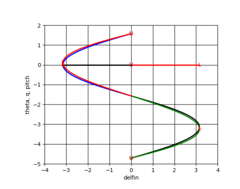
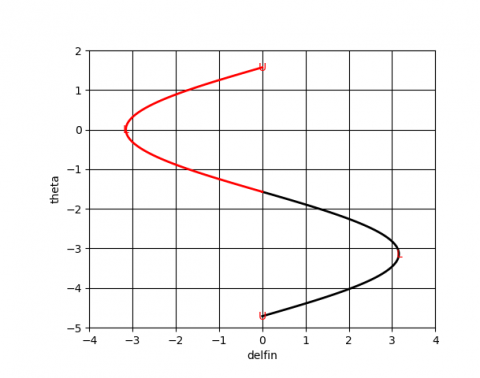
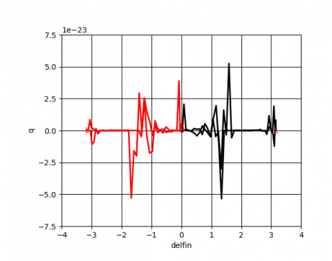
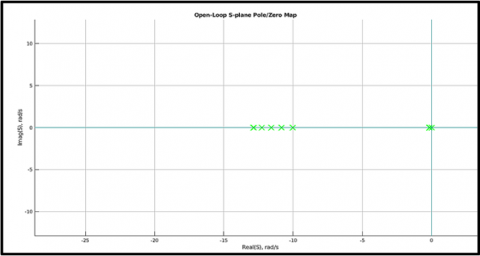
The method is implemented for the 3DOF longitudinal hybrid airship model by applying SBA for the nonlinear dynamic model [4, 7] and the state variables are given by x=[V, γ, α, θ, q, h]′. The states are further reduced for simplicity, considering constant velocity, V, constant height, h and considering very small changes in γ, thus the state variable considered for the analysis is reduced and is given by x=[α, θ, q]′. The SBA for the hybrid airship is implemented and bifurcation diagram with Eigen values for each case is obtained which shows the flight dynamics behaviours. The bifurcation diagram for velocity 20 m/s having mass of the vehicle as 10kg is shown in Figure 16. The stability information can be examined for the longitudinal dynamic model using Eigenvalues obtained from the bifurcation analysis. The system behaviour might be stable or unstable depending on these Eigenvalues. The different Eigenvalues obtained using the bifurcation method for the different cases with elevator deflection is shown in Table 5. The Eigenvalues obtained are used to plot the pole-zero map to understand the system stability behaviour and are shown in the Figure 17. The poles plot for the different simulation cases shows that Cases 1, 2, 3, 5 and 6 show stable behaviour and Cases 4 and 7 show unstable behaviour due to the poles lying on the RHS plane.
Table 5. Eigen values obtained using Bifurcation method
|
Simulation Cases |
Elevator deflection (delfin, deg) |
Eigenvalues |
Stability |
|
1 |
0.0 |
-0.195248, -11.5970, -44591.4 |
Stable |
|
2 |
1.5 |
-0.168959, -12.2705, -44591.2 |
stable |
|
3 |
3.13672 |
-0.00909272, -12.8659, -44591.0 |
Stable |
|
4 |
3.15437 |
0.000000092, -12.8647, -44591.0 |
Unstable |
|
5 |
-1.5 |
-0.168893, -10.8492, -44591.6 |
stable |
|
6 |
-3.13478 |
-0.00923439, -10.0340, -44591.8 |
stable |
|
7 |
-3.15253 |
0.0000000976266, -10.0296, -44591.8 |
Unstable |
(a)
(b)
(c)
(d)
Figure 16. Bifurcation diagram: (a) theta, q, pitch (combined); (b) θ in degree; (c) q in degree; (d) pitch vs dele deflection in degree
Figure 17. System poles plot for the simulation cases
The study presents the longitudinal trim with stability assessment of the 3DOF and 4DOF longitudinal hybrid airship model with dynamic simulation and stability analysis using the bifurcation method. Trim analysis and simulation of the 3DOF hybrid airship model are performed under the different cases of elevator deflections. For the different 7 cases, trim simulation is performed with the hybrid airship model resulting in the stable simulation for cases 1, 2, 3, 5 and 6 for elevator deflection δe=0 degree, δe=1.5 degree, δe=-1.5 degree, δe=3.13672 degree and δe=-3.13672 degree and for cases 4 and 7 for for elevator deflection δe=3.15437 and δe=-3.15437 show unstable behavior. The validation of the cases is carried out with the bifurcation method implementation using the 3DOF hybrid airship model with constant velocity and for level flight. Using the bifurcation method, for all the different cases, the eigenvalues are obtained, and corresponding poles are determined, and this shows and confirms the same findings for stable cases and unstable cases. The first longitudinal mode is the surge mode, and it is characterized by the drag variation due to speed. Since the drag variation due to speed is increased, the surge mode demonstrated by the winged hybrid airship is stable with small time constant of 0.442s. Two stable and one unstable mode obtained in longitudinal dynamics of a hybrid airship. The bifurcation analysis results presented here to demonstrate a potential way for determining the stability of different trim points. With the alternate model as two body longitudinal dynamics model i.e., 4DOF model, it is also suggested the same findings of trim condition as vel is 20m/s, gamma and theta as 0. MATLAB simulates the dynamic model using numerical integration as Runge–Kutta method where as AUTO for bifurcation method using continuation algorithm from one equilibrium to another equilibrium point. For 3DOF basic equation of motion of hybrid airship mathematical background is discussed and simulated. For developing the 3DOF model of hybrid, Centre of gravity and Centre of volume is distinctly located whereas in the alternate two body dynamics model this condition is not required, only suspended payload length from the vehicle is taken care. In all the model the same trim conditions are obtained. Velocity change is due to small disturbances in level flight. These oscillations can help us to study the dynamics of the vehicle under small disturbances. The obtained results will be used in designing a controller for making a real flight of the hybrid airship [29] with suspended payload vehicle. For creating a wireless zone, the proposed airship can be used as discussed in research [30].
[1] Khoury, G.A. (Ed.). (2012). Airship Technology (Vol. 10). United Kingdom: Cambridge University Press.
[2] Ardema, M.D. (1977). Feasibility of modern airships: Preliminary assessment. Journal of Aircraft, 14(11): 1140-1148. https://doi.org/10.2514/3.58902
[3] Prakash, O., Daftary, A., Ananthkrishnan, N. (2005). Bifurcation analysis of parafoil-payload system flight dynamics. In AIAA Atmospheric Flight Mechanics Conference and Exhibit, p. 5806. https://doi.org/10.2514/6.2005-5806
[4] Prakash, O., Daftary, A., Ananthkrishnan, N. (2005). Trim and stability analysis of parafoil/payload system using bifurcation methods. In 18th AIAA Aerodynamic Decelerator Systems Technology Conference and Seminar, p. 1666. https://doi.org/10.2514/6.2005-1666
[5] Sinha, N.K., Ananthkrishnan, N. (2014). Elementry Flight Dynamics with an Introduction to Bifurcation and Continuation Methods. FL, USA, CRC Press.
[6] Prakash, O., Purohit, S. (2022). Modeling and simulation of turning flight of winged airship-payload system using 9-DOF multibody model. In AIAA AVIATION 2022 Forum, p. 3422. https://doi.org/10.2514/6.2022-3422
[7] Prakash, O. (2020). Multibody dynamics of winged hybrid airship payload delivery system. In AIAA Aviation 2020 Forum, p. 3200. https://doi.org/10.2514/6.2020-3200
[8] Tiwari, A., Vora, A., Sinha, N.K. (2016). Airship trim and stability analysis using bifurcation techniques. In 2016 7th International Conference on Mechanical and Aerospace Engineering (ICMAE), London, UK, pp. 471-475. https://doi.org/10.1109/ICMAE.2016.7549586
[9] Prakash, O., Kumar, A. (2022). NDI based Heading Tracking of Hybrid-Airship for payload delivery. In AIAA SCITECH 2022 Forum, p. 1432. https://doi.org/10.2514/6.2022-1432
[10] Singh, R., Prakash, O., Joshi, S., Jeppu, Y. (2022). Bifurcation analysis of longitudinal dynamics of generic air-breathing hypersonic vehicle for different operating flight conditions. In: Banerjee, S., Saha, A. (eds) Nonlinear Dynamics and Applications. Springer Proceedings in Complexity. Springer, Cham. https://doi.org/10.1007/978-3-030-99792-2_97
[11] Prakash, O., Singh, R. (2021). Flight dynamics analysis using high altitude & Mach number for generic air-breathing hypersonic vehicle. In AIAA Propulsion and Energy 2021 Forum, p. 3271. https://doi.org/10.2514/6.2021-3271
[12] Prakash, O., Ananthkrishnan, N. (2006). Modeling and simulation of 9-DOF parafoil-payload system flight dynamics. In AIAA Atmospheric Flight Mechanics Conference and Exhibit, p. 6130. https://doi.org/10.2514/6.2006-6130
[13] Zhang, K.S., Han, Z.H., Song, B.F. (2010). Flight performance analysis of hybrid airship: Revised analytical formulation. Journal of Aircraft, 47(4): 1318-1330. https://doi.org/10.2514/1.47294
[14] Mackrodt, P.A. (1980). Further studies in the concept of delta-winged hybrid airships. Journal of Aircraft, 17(10): 734-740. https://doi.org/10.2514/3.57960
[15] Verma, A.R., Sagar, K.K., Priyadarshi, P. (2014). Optimum buoyant and aerodynamic lift for a lifting-body hybrid airship. Journal of Aircraft, 51(5): 1345-1350. https://doi.org/10.2514/1.C032038
[16] Nagabhushan, B.L. (1983). Dynamic stability of a buoyant quad-rotor aircraft. Journal of Aircraft, 20(3): 243-249. https://doi.org/10.2514/3.44859
[17] Kumar, A., Prakash, O. (2022). Nonlinear modelling and analysis of longitudinal dynamics of hybrid airship. In: Banerjee, S., Saha, A. (eds) Nonlinear Dynamics and Applications. Springer Proceedings in Complexity. Springer, Cham. https://doi.org/10.1007/978-3-030-99792-2_82
[18] Andan, A.D., Asrar, W., Omar, A.A. (2012). Investigation of aerodynamic parameters of a hybrid airship. Journal of Aircraft, 49(2): 658-662. https://doi.org/10.2514/1.C031491
[19] Kumar, A., Prakash, O. (2022). Analysis of lateral dynamics of ARX model of an aircraft with model predictive controller. In 2022 International Conference for Advancement in Technology (ICONAT), Goa, India, pp. 1-6. https://doi.org/10.1109/ICONAT53423.2022.9726117
[20] Ashraf, M.Z., Choudhry, M.A. (2013). Dynamic modeling of the airship with Matlab using geometrical aerodynamic parameters. Aerospace Science and Technology, 25(1): 56-64. https://doi.org/10.1016/j.ast.2011.08.014
[21] Acanfora, M., Lecce, L. (2016). On the development of the linear longitudinal model for airships stability in heaviness condition. Aerotecnica Missili & Spazio, 90(1): 33-40.
[22] Doedel, E J., Champneys, A.R., Dercole, F., Fairgrieve, T.F., Kuznetsov, Y.A., Oldeman, B., Paffenroth R.C., Sandstede B., Wang X.J., Zhang, C.H. (2007). AUTO-07P: Continuation and bifurcation software for ordinary differential equations. Department of Computer Science, Concordia University, Montreal, Canada.
[23] Roskam, J. (1971). Methods for estimating stability and control derivatives of conventional subsonic airplanes. University of Kansas, Lawrence, Kansas.
[24] Campbell, J.P., McKinney, M.O. (1951). Summary of methods for calculating dynamic lateral stability and response and for estimating lateral stability derivatives (No. NACA-TN-2409).
[25] Nelson, R.C. (1998). Flight Stability and Automatic Control (Vol. 2). New York: WCB/McGraw Hill.
[26] Yechout, T.R. (2003). Introduction to Aircraft Flight Mechanics. Aiaa. Virginia: AIAA Education Series.
[27] Slegers, N., Costello, M. (2003). Aspects of control for a parafoil and payload system. Journal of Guidance, Control, and Dynamics, 26(6): 898-905. https://doi.org/10.2514/2.6933
[28] Kamman, J.W., Huston, R.L. (2001). Multibody dynamics modeling of variable length cable systems. Multibody System Dynamics, 5: 211-221. https://doi.org/10.1023/A:1011489801339
[29] De Busk, W., Johnson, E., Chowdhary, G. (2009). Real-time system identification of a small multi-engine aircraft. In AIAA Atmospheric Flight Mechanics Conference, p. 5935. https://doi.org/10.2514/6.2009-5935
[30] Kafafy, R., Okasha, M., Alblooshi, S., Almansoori, H., Alkaabi, S., Alshamsi, S., Alkaabi, T. (2022). A remotely-controlled micro airship for wireless coverage. Applied Research and Smart Technology (ARSTech), 3(2): 72-80. https://doi.org/10.23917/arstech.v3i2.1190