Nitin Kumar Mishra![]() | Sakshi Sharma*
| Sakshi Sharma*![]()
© 2023 IIETA. This article is published by IIETA and is licensed under the CC BY 4.0 license (http://creativecommons.org/licenses/by/4.0/).
OPEN ACCESS
The main contribution of this article is to inspect the role of variable inflation rate in every replenishment cycle in supply chain management. An inventory, time, and inflation-dependent demand are contemplated. Some completely novel concepts are introduced. Inflation and its effect are studied in every single replenishment cycle, furthermore, equipoise is attained under a single supplier – multiple retailers’ coordination in a highly dynamic and competitive free market. Moreover, the equipoise cost of the retailer is used to ultimately reduce the costs of both the supplier and retailers. The algorithms are discussed in detail to understand the working of our new model, which is close to real-world based problems encountered in inventory management. Numerical examples are discussed in support of theoretical aspects mentioned with the help of Mathematica software 12.0.
equipoise, trade credit, FMCG, single supplier, multiple retailers, variable inflation rate
Inflation is the result of a greater supply of money than its demand. Greater demand than supply, leads to inflationary conditions in an economy. Buzacott [1] was the first researcher who wrote something about inflation in inventory models by formulating a minimum cost model for a single item in inventory and studied the effect of inflation. Guria et al. [2] framed an inventory policy for an item with inflation and demand depending on the selling price by adding a new parameter of immediate part payments to the wholesaler. In 1985, Goyal [3] gave an EOQ model with permissible delays in payments. Later in 1995, Aggarwal and Jaggi [4] extended their work and gave a relation between sales revenue and delay period along with the rate of interest. Supplier-Retailer coordination/setup is taken up by innumerable researchers. Esmaeili and Nasrabadi [5] in 2020 talked about the single vendor-multiple retailers set up.
Thusly, the main contribution of this article is to examine the role of variable inflation rates in inventory management. The main reason behind considering the variable inflation in each replenishment cycle is the competitive and fast changing scenario exiting in the present world and as a result, the prices rise faster as compared to earlier. A supplier with multiple retailers’ setups is considered. Equipoise of total inventory cost for multiple retailers in a given competitive environment is calculated. The supplier and multiple retailers' trade credits are considered and the process is controlled by the supplier showing the well-coordinated supply chain management. As per our literature review, the variable inflation per cycle is not taken into account by any researcher.
Well, there is a lot to discuss in the literature review, here we will consider those research articles only which are related to the scope of our research. Till now, much has been talked about factors that impact the cost and profit of a supplier and a retailer. Demand patterns, deterioration, trade credit, shortages, availability of raw material, transportation cot, set up cost, holding cost, purchase cost, ordering cost, lost sales, opportunity cost, labor cost, machinery cost, inflation, seasonal patterns of a product and many more are all pillars that need to be studied well to make a model in inventory management that reduces cost or maximizes the profit of a supplier or retailer or the whole system. Inventory-led and time-led demand is such, which can’t be overlooked to tackle inventory management paraphernalia. Inventory managers can’t neglect the impact and after-effects of inflation, and the dynamic nature of inflation is the most cumbersome thing to be taken care of. In a market where there are high inflationary conditions and dynamic forces are most active, coordination among the players of the market can highly affect some important costs related to the inventory system. In the futuristic and promising industry of FMCG, everything is or will be found, which is included in Inventory Management System.
In 2009, Mirzazadeh et al. [6] in their inventory model, under finite production rate talked about an uncertain inflationary setup. In 2011, Tripathi [7] discussed important parameters of pricing and ordering policy under inflation with permissible delay in payments. In 2013, Shastri et al. [8] added manufacturers along with suppliers and retailers for deteriorating items in inflationary situations. Weibull Deterioration is added by Singh and Panda [9] in 2015 along with the above-taken parameters. In 2015 itself, Kiniwa et al. [10] added deflation in the price stabilization process. In 2020, Geetha and Udayakumar [11] wrote about deteriorating items along with inflation-induced demand which was time-dependent as well in infinite horizon. In 2020, Sundararajan et. al. [12] studied the impact of delays in payments along with shortages and inflation. In 2021, Sundararajan et. al. [13] gave price determination along with the deterioration of items under inflation and delay in payments. Alterations are always perceived in inflation, under the impact of numerous dynamic constituents, thusly we can't take inflation in inventory as constant or the same throughout the horizon.
So far, researchers have different present coordination between the supplier and the retailer. Guria et al. [2], An inventory control system is developed in which immediate part payment is allowed and permissible delay in payments is also allowed for the rest of the period by the wholesaler for an item over a finite planning horizon or random planning horizon. Moreover, demand taken is inflation and selling price dependent. Chung et al. [14] presented inventory models and discuss the case that at what time the retailer will prefer cash discounts and when they will go for trade credits. Zhong et al. [15], 2017 proposed an integrated location and two-way inventory networking model in consideration of trade credit. Mahato et al. [16] in 2021, gave two step supply chain under trade credit considering the hybrid price and stock depending demand and concluded that centralized policy will give more profits. In 2021, Mandal et al. [17] gave advertisement and stock level dependent inventory models under trade credit policy with deterioration rate as a constant function of on-hand inventory.
Wu and Zhao [18] in 2014, emphasized supplier-retailer coordination along with trade credit period rate in a finite planning horizon. Their model is even applicable for consumer packaged goods or FMCG. In 2017, Singh et al. [19] presented an EOQ model in a finite planning horizon for two cases-with and without delay in payments. In 2018 again, Singh et al. [20] gives an inflation-based inventory model in a finite planning horizon including trade credit. In 2019, Singh et al. [21] under a centralized and decentralized planning horizon incorporated trade credit policy as well. In 2020, Esmaeili and Nasrabadi [5] takes the coordination between a supplier and a retailer a step forward by giving a single supplier and multiple retailer model under the impact of inflation and trade credit. Taghizadeh-Yazdi et al. [22] gave an integrated inventory model, considering coordination among suppliers-manufacturer-distributor, and proves that profits raised by 15%.
Thus far, dissimilar demands were taken into account for developing profuse inventory models. To name a few, inventory-dependent, time-led demand, selling price demand, inflation-induced demand, stock-dependent demand, etc. were an inseparable part of supply chain management-associated research from years on end. Liao et al. [23] gave an inventory model stock-dependent consumption rate under permissible delay in payments. In 2014 model by Wu and Zhao [18], took inventory and time-dependent demand. In 2015, Kumar and Rajput [24], worked on time and stock-dependent demand along with inflation and credit policy. Saha and Sen [25] added selling price-dependent demand along with time dependency in their inflation-based optimal inventory model. Shaikh et al. [26] added partial backlogging and deteriorating items along with stock-led demand in the EOQ model with the facility of price discount. Barman et al. [27] added variable and cloud fuzzy demand rates with inflation in their inventory model. Khan et al. [28] gave a supply chain model with a non-linear stock-dependent demand rate.
The FMCG sector is a fast emerging sector. These Consumer Packaged Goods (CPG) are inexpensive merchandise that sells quickly. This industry is mainly responsible for producing, distributing, and even marketing these CPG. Nemtajela and Mbohwa [29] proved that there is a direct relation between managing inventory levels and uncertainty of demand i.e., more the uncertainty levels of demand, the inventory managers need to deal with more cumbersome inventory management problems for FMCG. Jaggi et al. [30] explained that consumer goods or products with displayed stocks need to have a centralized policy for achieving maximum joint profit by both the supplier and the retailer, though the profits are biased for the retailer. In 2020, Li et al. [31] in their work explained how the inventory can be optimized for fast-moving consumer products by replenishing and salvaging the stocks at the start of each cycle by focusing on the e-commerce platform for promoting these consumer packaged goods.
Table 1. A comparison of the inventory models
|
Author(s) Name & Year |
Inflation |
Horizon |
Coordination |
Trade Credit |
FMCG |
|
Mirzazadeh et al. [6] |
Stochastic |
Finite |
S-R |
No T.C |
No |
|
Tripathi [7] |
Constant |
Infinite |
S-R |
IE-IC |
No |
|
Shastri et al. [8] |
Constant |
Infinite |
S-M-R |
No T.C |
No |
|
Singh and Panda [9] |
Constant |
Finite |
S-R |
IE-IC |
No |
|
Singh et al. [19] |
Constant |
Finite |
S-R |
Avg. (min, max.) |
No |
|
Singh et al. [21] |
No |
Finite |
S-R |
Profit sharing |
No |
|
Esmaeili and Nasrabadi [5] |
Discrete- Time Markov Chain |
Fixed |
S-Multiple retailers |
IE-IC |
No |
|
Sundararajan et al. [12] |
Constant |
Infinite |
S-R |
IE-IC (single level) |
No |
|
Sundararajan et al. [13] |
Constant |
Infinite |
S-R |
IE-IC (single level) |
No |
|
Geetha and Udayakumar [11] |
Constant |
Infinite |
S-R |
No T.C |
No |
|
Present Paper |
Exponential & Variable in each replenishment cycle |
Finite |
S-Multiple retailers |
Equipoise |
Yes |
S-Supplier, R-Retailer, M-Manufacturer, IE-Interest Earned, IC-Interest Charged, T.C.-Trade Credit.
Table 1 specifies that inflation is considered constant quite a lot of times. Coordination between supplier and retailer is maximum time based on trade credit policy or credit period policy based on interest earned and interest charged. Though Esmaeili and Nasrabadi [5] moved out of the box and consider the Discrete-Time Markov Chain inflation rate, they discussed two cases of the inflation rate, one with Discrete-Time Markov Chain and the other without Discrete-Time Markov Chain. They even consider single vendor-multiple retailers set up, but coming on to credit period, once again they went back to traditional interest charged and interest earned concept. The last column is for the models which apply to FMCG.
Some noticeable considerations of our research article are: (i) variable inflation is considered in all replenishment cycles. (ii) The finite planning horizon is taken. (iii) Single supplier-multiple retailers set up is undertaken. (iv) Equipoise is discussed for a total cost of each retailer in coordination with the supplier and then the credit period is offered based on equipoise cost. (v) The model introduced in this article applies to all the products encompassed in the FMCG industry. All the novel concepts introduced are necessary to run the machinery of the FMCG sector smoothly.
In this piece of writing, the effect of inflation is studied at every step. The main reason behind doing all this is to see how inflation affects the prices or cost, when inflation rises every time, the inventory get replenished. We have considered a linear rise in inflation which no one has taken before this, making our work a novel piece. The coordination between the supplier and the retailer has been taken to a different level. Using the coordination between the two, the retailer's cost equipoise has been worked out. The biggest advantage to the market (more precisely to the consumer) from this would be that the price of a product would remain the same with every retailer, that too when the deep analysis and effect of inflation has been considered. Retailer’s cost equipoise is an unconventional concept in inventory management.
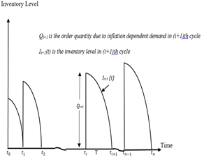
The supplier takes an order from a retailer at time t0=0, the inventory level reaches zero at t1 and then the inventory is refilled instantaneously. No shortages or deterioration rate is considered, as the targeted field is FMCG. Inventory and time-dependent demand along with inflation-based demand are considered. The model and its graphical representation are shown in Figure 1, where t0 is zero and the horizon is finite. Ii+1(t) depicts the inventory level in (i+1)th cycle.
Figure 1. Graphical representation of the model
Case 1: When there is no coordination between the supplier and the retailers.
The differential equation of the inventory level in (i+1)th cycle will be given as follows:
$\begin{gathered}\frac{d I_{i+1}(t)}{d t}+k I_{i+1}(t)=-\left(b_1 t+b_2 e^{\alpha_i t}\right), t_i \leq t \leq t_{i+1}\end{gathered}$ (1)
where, boundary conditions are Ii+1(ti+1)=0 and Ii(ti)=Qi+1. Therefore, the solution of Eq. (1) is.
$\begin{gathered}I_{i+1}(t)=e^{-k t} \int_t^{t_{i+1}} e^{k u}\left(b_1 u+b_2 e^{\alpha_i u}\right) d u \,\,t_i \leq t \leq t_{i+1}\end{gathered}$ (2)
Refer to Appendix A for the solution to Eq. (1).
The order quantity for (i+1)th cycle is:
$Q_{i+1}=I_{i+1}\left(t_i\right)=e^{-k t_i} \int_{t_i}^{t_{i+1}} e^{k t}\left(b_1 t+b_2 e^{\alpha_i t}\right) d t$
$such \,that$, $u \in\left[t, t_{i+1}\right]$ and $t_i \leq t \leq u \leq t_{i+1}$ (3)
The ordering cost of the retailer is:
$Y\left(\sum_{j=0}^{n-1}\left(\left(e^{\sum_{i=0}^j \alpha_{i+1}\left(t_{i+1}-t_i\right)}\right)\right)\right)$ (4)
Refer to Appendix B for the solution to Eq. (4).
The holding cost of the retailer is:
$\begin{aligned} & \left(\sum_{j=0}^{n-1}\left(\left(e^{\sum_{i=0}^j \alpha_{i+1}\left(t_{i+1}-t_i\right)}\right) * \frac{1}{2 k^3} b_1\left(2-2 e^{k\left(-t_j+t_{1+j}\right)}-2 k t_j\right.\right.\right. \\ & \left.+k^2 t_j^2+2 e^{k\left(-t_j+t_{1+j}\right)} k t_{1+j}-k^2 t_{1+j}^2\right) \\ & \left.+\frac{b_2\left(\frac{e^{-k t_j+t_{1+j} \alpha_{1+j}}\left(-e^{k t_j}+e^{k t_{1+j}}\right)}{k}+\frac{e^{t_j \alpha_{1+j}}-e^{t_{1+j} \alpha_{1+j}}}{\alpha_{1+j}}\right)}{k+\alpha_{1+j}}\right)\end{aligned}$ (5)
Refer to Appendix C for the solution to Eq. (5).
The purchasing cost of the retailer is:
$\begin{aligned} & \left(W\left(\sum_{j=0}^{n-1}\left(\left(e^{\sum_{i=0}^j \alpha_{i+1}\left(t_{i+1}-t_i\right)}\right) *\left(b_1\left(\frac{e^{k\left(t_{j+1}-t_j\right)} * t_{j+1}}{k}\right.\right.\right.\right.\right. -\frac{e^{k\left(t_{j+1}-t_j\right)}}{k^2}-\frac{t_j}{k}+\frac{1}{\left.k^2\right)} \\ & \left.\left.\left.+b_2\left(\frac{e^{\alpha_{j+1} * t_{j+1}} * e^{k\left(t_{j+1}-t_j\right)}-e^{t_j^* \alpha_{j+1}}}{k+\alpha_{j+1}}\right)\right)\right)\right) \\ & \end{aligned}$ (6)
Refer to Appendix D for the solution to Eq. (6).
The retailer’s total cost will be the sum of ordering cost, holding cost, and purchasing cost.
Adding Eqns. (4), (5), and (6), we get:
$\begin{aligned} & R_I =W\left(\sum_{i=0}^{n-1}\left(\left(e^{\sum_{i=0}^j \alpha_{i+1}\left(t_{i+1}-t_i\right)}\right) *\left(b_1\left(\frac{e^{k\left(t_{j+1}-t_j\right)} * t_{j+1}}{k}\right.\right.\right.\right. \left.-\frac{e^{k\left(t_{j+1}-t_j\right)}}{k^2}-\frac{t_j}{k}+\frac{1}{k^2}\right) \left.\left.+b_2\left(\frac{e^{\alpha_{j+1} * t_{j+1}} * e^{k\left(t_{j+1}-t_j\right)}-e^{t_j^* \alpha_{j+1}}}{k+\alpha_{j+1}}\right)\right)\right) \\ & +Y\left(\sum_{j=0}^{n-1}\left(\left(e^{\sum_{i=0}^j \alpha_{i+1}\left(t_{i+1}-t_i\right)}\right)\right)\right) +h\left(\sum_{i=0}^{n-1}\left(\left(e^{\sum_{i=0}^j \alpha_{i+1}\left(t_{i+1}-t_i\right)}\right) * \frac{1}{2 k^3} b_1\left(2-2 e^{k\left(-t_j+t_{1+j}\right.}\right)\right.\right. \left.-2 k t_j+k^2 t_j^2+2 e^{k\left(-t_j+t_{1+j}\right)} k t_{1+j}-k^2 t_{1+j}^2\right) \\ & \left.+\frac{b_2\left(\frac{e^{-k t_j+t_{1+j} \alpha_{1+j}}\left(-e^{k t_j}+e^{k t_{1+j}}\right)}{k}+\frac{e^{t_j \alpha_{1+j}}-e^{t_{1+j} \alpha_{1+j}}}{\alpha_{1+j}}\right)}{k+\alpha_{1+j}}\right) \\ & \end{aligned}$ (7)
Let $n^*, t_1^*, t_2^*, \ldots, t_{n-1}^*$ be the optimal solution for the minimum total cost of the retailer (RI). Under this first case, of no coordination supplier’s cost will be affected by the retailer’s replenishment rate. The supplier’s total cost will be the sum of set up cost and manufacturing cost.
Set-up cost is a further sum of Labour Cost (LC) and Machinery Cost (MC).
$\begin{aligned} S_I\left(n^*, t_0, t_1^*, t_2^*, \ldots\right. & \left.t_{n-1}^*\right) =\left(n^*-1\right)(L C+M C) +\sum_{j=0}^{n^*-1} c * Q_{j+1}^*\end{aligned}$ (8)
The total order quantity during the planning horizon is:
$Q_I=\sum_{j=0}^{n^*-1} Q_{j+1}^*$ (9)
Algorithm 1 for Case 1: (In case of no coordination)
Step 1: To find the optimal schedule for ordering from the retailer.
Step 1 (i): Assign n=2, 3, 4, and so on.
Step 1 (ii): Solve Eq. (10) for n=2, 3, 4 and so on.
Step 1 (iii): Derived values of t0, t1, t2, and so on will be used to calculate the value of the total cost of the retailer from Eq. (7).
Step 2: Find the optimal replenishment cycle.
Step 3: Use the optimal replenishment cycle value derived in the previous step to calculate the optimal cost of the supplier from Eq. (8) and the total quantity from Eq. (9).
Case 2: When there is coordination among the supplier and multiple retailers.
Credulous arrangement for competitive market model
Our system for Case 2 constitutes a set of retailers with different costs of the product. The intent behind fabricating this arrangement is to reach an equipoise, in inventory cost of retailers under the assistance of the supplier (at two phases, to achieve equipoise and thenceforth deciding credit period).
Let Mi, i=1,2,3,4,…. be the set of nabe retailers with dissimilar inventory costs at the initial step. Here we presume, that each retailer has goods and in the initial phase has different inventory costs. Under the defined array, a pair of retailers will be undertaken that have maximum and minimum inventory costs of the product. The inventory cost of each retailer will be designated as $C_{R_i}$, i=1,2,3,… to calculate the inventory cost of each retailer, we follow below mentioned procedure.
The inventory cost of the retailers is calculated from Eq. (7). The unit cost of the product is given by dividing the solutions obtained from Eq. (7) by the solutions of Eq. (9). This particular unit cost of the product will be different for all the retailers in the market (keeping in mind the variable holding cost, ordering cost, and purchasing cost of the retailer initially). The supplier will contact the retailers and will give them trade credits for bringing their cost up to equipoise in the competitive free market.
Proffer design
In this section, we consider an arrangement most appropriate for FMCG competitive market. Under this, unabridged procedure, RATProffer is initiated, in which each retailer will always proffer another nabe retailer with the lowest cost of the product, where cost is always an integer.
RATProffer
Each retailer, $C_{R_i}, i=1,2,3, \ldots$. proffer $\quad C_{R_{i j}}=C_j+$ $\left(\frac{C_i-C_j}{z}\right)$ where $z \geq 1, \quad i, j \in M_i$, to another retailer $C_{R_i}, i=$ $1,2,3, \ldots \ldots \in M_i$ by using the formula defined by the above-mentioned formula. For calculating equipoise of Inventory Cost for Multiple Retailers in a given Competitive Environment the following algorithm will be followed:
Algorithm 2 for Case 2:
Step 1: Under the coordination case, use the value derived in step 1 (c) (from Algorithm 1) of the total cost of the retailer and the value of total quantity from Step 1 (e) (from Algorithm 1) divide the total cost of a retailer with the quantity of the product to evaluate the per unit cost of the product for one retailer.
Step 2: Repeat Step 1 for 4 retailers.
Step 3: Consider the values per unit cost of the product for Retailers as C1, C2, C3, C4.
Step 3 (a): Find the largest among the four values of C1, C2, C3, C4.
Step 3 (b): Find the smallest among the four values of C1, C2, C3, C4.
Step 3 (c): When C1 is largest and C2 is smallest, Replace C2 with S, and calculate S+(C1-S)/z and replace C1= C2=S.
Step 3 (d): Repeat Step 3 (c) when C1 is largest and C3 is smallest by replacing C2 with C3.
Step 3 (e): Repeat Step 3 (c) when C1 is largest and C4 is smallest by replacing C2 with C4.
Step 3 (f): When C2 is largest and C1 is smallest, calculate VC1 C2=C1+((C2-C1)/z) and assign C1=C2=VC1 C2.
Step 3 (g): Repeat Step 3 (e) when C2 is largest and C3 is smallest by replacing C1 with C3.
Step 3 (h): When $C_3$ is largest and $C_1$ is smallest, calculate $V C_1 C_3=C_1+\left(\frac{C_3-C_1}{z}\right)$ and replace C1=C3=VC1 C3
Step 3 (i): Repeat Step 3 (h) when C3 is largest and C2 is smallest by replacing C1 with C2.
Step 3 (j): If C1=C2=C3=C4 then the equipoise is achieved and the program ends, if no then go to Step 3 (a).
Once the equipoise is attained, it meant that all retailers now have the same inventory cost for a product, no matter how many different costs a retailer had at the preliminary stage. The retailer whose cost was greater than the equipoise earlier, this meant that he would be given compensation in terms of interest through the trade credit facility offered by the supplier whereas the retailer whose cost was prior less than the equipoise, would automatically benefit from the increased equipoise cost.
Definition 1: (Tenable Layout). A layout is tenable if the cost of the product for different retailers is the same.
Definition 2: (CostPact). A pact between two retailers during the execution of RATProffer.
Theorem 1: The layout RATProffer is without any stalemate point. This implies that there prevails some inventory cost in Mi considering the layout to be tenable.
Proof: Refer to Appendix E.
Theorem 2: The layout in due course will reach equipoise.
Proof: Refer to Appendix F.
To determine the optimality of the replenishment schedule.
To resolve the optimality of the replenishment schedule, from Eq. (7) of the total cost of the retailer we will calculate $\frac{\partial R_I}{\partial t_i}$ and then put $\frac{\partial R_I}{\partial t_i}=0$ where i=1, 2, 3, ……n-1. Since we are working on multiple retailers set up, the optimality will be for all the retailers individually. We will be proving for RI2 and will be the same for all the other retailers.
$\begin{aligned} & \frac{\partial \mathrm{R}_{\mathrm{I} 2}}{\partial \mathrm{t}_{\mathrm{i}}}=\mathrm{h}\left\{\left(\alpha_{\mathrm{i}}-\alpha_{1+\mathrm{i}}\right) *\left(\mathrm{e}^{\sum_{\mathrm{i}=0}^{\mathrm{j}} \alpha_{\mathrm{i}+1}\left(\mathrm{t}_{\mathrm{i}+1}-\mathrm{t}_{\mathrm{i}}\right)}\right) *\right. \left(\frac{1}{2 \mathrm{k}^3} \mathrm{~b}_1\left(2-2 \mathrm{e}^{\mathrm{k}\left(-\mathrm{t}_{\mathrm{j}}+\mathrm{t}_{1+\mathrm{j}}\right)}-2 \mathrm{kt}_{\mathrm{j}}+\mathrm{k}^2 \mathrm{t}_{\mathrm{j}}^2+\right.\right. \left.2 e^{\mathrm{k}\left(-\mathrm{t}_{\mathrm{j}}+\mathrm{t}_{1+\mathrm{j}}\right)} \mathrm{kt}_{1+\mathrm{j}}-\mathrm{k}^2 \mathrm{t}_{1+\mathrm{j}}^2\right)+ \\ & \left.\frac{b_2\left(\frac{e^{-k_j+t_{1+j} \alpha_{1+j}}\left(-e^{k t_j}+e^{k t_1+j}\right)}{k}+\frac{e^{t_j \alpha_{1+j}}-e^{t_{1+j} \alpha_{1+j}}}{\alpha_{1+j}}\right)}{k+\alpha_{1+j}}\right)+ \left(\mathrm{e}^{\sum_{\mathrm{i}=0}^{\mathrm{j}} \alpha_{\mathrm{i}+1}\left(\mathrm{t}_{\mathrm{i}+1}-\mathrm{t}_{\mathrm{i}}\right)}\right) * \frac{\left(-\mathrm{e}^{\mathrm{k}\left(-\mathrm{t}_{-1+\mathrm{i}}+\mathrm{t}_{\mathrm{i}}\right)} \mathrm{k}+\mathrm{e}^{\mathrm{k}\left(-\mathrm{t}_{\mathrm{i}}+\mathrm{t}_{1+\mathrm{i}}\right)} \mathrm{k}\right) \mathrm{b}_1}{\mathrm{k}^3}\\&+ \frac{\mathrm{b}_1\left(-1+e^{\mathrm{k}\left(-\mathrm{t}_{-1+i}+\mathrm{t}_{\mathrm{i}}\right)}+\mathrm{e}^{\mathrm{k}\left(-\mathrm{t}_{-1+i}+\mathrm{t}_{\mathrm{i}}\right)} \mathrm{kt}_{\mathrm{i}}-\mathrm{e}^{\mathrm{k}\left(-\mathrm{t}_{\mathrm{i}}+\mathrm{t}_{1+\mathrm{i}}\right)} \mathrm{kt}_{1+\mathrm{i}}\right)}{\mathrm{k}^2}+ \end{aligned}$
$\begin{aligned} & \frac{\mathrm{e}^{\mathrm{k}\left(-\mathrm{t}_{-1+\mathrm{i}}+\mathrm{t}_{\mathrm{i}}\right)+\mathrm{t}_{\mathrm{i}} \alpha_{\mathrm{i}_2}}}{\mathrm{k}+\alpha_{\mathrm{i}}}+\frac{\mathrm{e}^{\mathrm{t}_{\mathrm{i}} \alpha_{\mathrm{i}} \mathrm{b}_2\left(-\frac{1}{\mathrm{k}}+\frac{\left.\mathrm{e}^{\mathrm{k}(-\mathrm{t}}-1+\mathrm{i}+\mathrm{t}_{\mathrm{i}}\right)}{\mathrm{k}}-\frac{1}{\alpha_{\mathrm{i}}}\right) \alpha_{\mathrm{i}}}}{\mathrm{k}+\alpha_{\mathrm{i}}}+\left.\frac{\mathrm{e}^{\mathrm{t}_{\mathrm{i}} \alpha_{1+\mathrm{i}} \mathrm{b}_2}}{\mathrm{k}+\alpha_{1+\mathrm{i}}}-\frac{\mathrm{e}^{\mathrm{k}\left(-\mathrm{t}_{\mathrm{i}}+\mathrm{t}_{1+\mathrm{i}}\right)+\mathrm{t}_{1+\mathrm{i}} \alpha_{1+\mathrm{i}} \mathrm{b}_2}}{\mathrm{k}+\alpha_{1+\mathrm{i}}}\right\}+ \\&\mathrm{Y}\left\{\mathrm{e}^{\sum_{\mathrm{i}=0}^{\mathrm{i}-1} \alpha_{\mathrm{i}+1}\left(\mathrm{t}_{\mathrm{i}+1}-\mathrm{t}_{\mathrm{i}}\right)} *\left(\alpha_{\mathrm{i}}-\alpha_{\mathrm{i}+1}\right)\right\}+ \mathrm{e}^{\sum_{\mathrm{i}=0}^{\mathrm{i}} \alpha_{\mathrm{i}+1}\left(\mathrm{t}_{\mathrm{i}+1}-\mathrm{t}_{\mathrm{i}}\right)} *\left(\alpha_{\mathrm{i}}-\alpha_{\mathrm{i}+1}\right) * \left(b_1\left(\frac{e^{k\left(t_{i+1}-t_i\right)_* t_{i+1}}}{k}-\frac{e^{k\left(t_{i+1}-t_i\right)}}{k^2}-\frac{t_i}{k}+\frac{1}{k^2}\right)+\right. \\ & \end{aligned}$
$\begin{aligned} & \mathrm{b}_2\left(\frac{\left.\mathrm{e}^{\alpha_{i+1} * \mathrm{t}_{i+1} * \mathrm{e}^{\mathrm{k}\left(\mathrm{t}_{\mathrm{i}+1}-\mathrm{t}_{\mathrm{i}}\right)}-\mathrm{e}^{\mathrm{t}_{\mathrm{i}} * \alpha_{i+1}}}\right)}{k+\alpha_{i+1}}\right)+ \mathrm{e}^{\sum_{\mathrm{i}=0}^{\mathrm{i}} \alpha_{i+1}\left(\mathrm{t}_{\mathrm{i}+1}-\mathrm{t}_{\mathrm{i}}\right)} *\left(\mathrm{~b}_1\left(-\frac{1}{\mathrm{k}}+\frac{\mathrm{e}^{\mathrm{k}\left(-\mathrm{t}_{\mathrm{i}}+\mathrm{t}_{1+\mathrm{i}}\right)}}{\mathrm{k}}-\right.\right. \left.\mathrm{e}^{\mathrm{k}\left(-\mathrm{t}_{\mathrm{i}}+\mathrm{t}_{1+\mathrm{i}}\right)} * \mathrm{t}_{1+\mathrm{i}}\right)+ \end{aligned}$
$\frac{b_2\left(-e^{k\left(-t_i+t_{1+i}\right)+t_{1+i^*} \alpha_{1+i}} k-e^{\left.t_i * \alpha_{1+i} \alpha_{1+i}\right)}\right.}{k+\alpha_{1+i}}))=0$ (10)
By using Eq. (10) the values of ti’s are obtained and finally, we calculate the total cost of the retailers. Next, we prove, Optimality of the replenishment cycle in Theorem 3.
Theorem 3: The unique solution to a nonlinear system of Eq. (10) derived by obtaining the first derivative of RI2is the optimal replenishment cycle length for a given n.
Proof: Refer to Appendix G for proof.
To illustrate our model, the following example is considered taking into account the above-mentioned assumptions under the Assumptions section.
Example: For four retailers: Given W=3, k=1.1, b1=40, b2=20, Y=500, α(1+i)=+0.01, i=1, 2, 3, ….,8, LC=30, MC=30, c=2, h1=0.0375, h2=0.05, h3=0.0625, h4=0.10, by applying algorithm 1 the values of Total cost of retailer is obtained and is shown in the Table 2 below:
Table 2. Total cost of all four retailers with different holding costs
|
Retailers |
Holding cost |
N=2 |
N=3 |
N=4 |
n=5 |
N=6 |
N=7 |
|
RI1 |
h1=0.0375 |
6762.30 |
328.28 |
2835.13 |
3680.48 |
4594.77 |
5590.03 |
|
RI2 |
h2=0.05 |
6761.65 |
327.89 |
2834.61 |
3679.49 |
4593.08 |
5587.36 |
|
RI3 |
h3=0.0625 |
6760.34 |
327.10 |
2833.56 |
3677.51 |
4589.72 |
5582.04 |
|
RI4 |
h4=0.10 |
6763.43 |
328.81 |
2836.87 |
3682.10 |
4595.56 |
5589.03 |
Table 2 depicts the total cost of four different retailers having variable holding costs in coloumn 2. The total cost is minimal when n=3. This results in obtaining the optimal replenishment interval at 3. Therefore, in this example the total cost function obtained is found to be convex. Now substituting these values, we will calculate the value of the total cost of the supplier (SI) concerning all four retailers which are tabled under Table 3 below.
Table 3. Total cost of Supplier concerning retailers
|
SRI1 |
SRI2 |
SRI3 |
SRI4 |
|
62397.9 |
62380 |
62344 |
62309.9 |
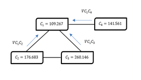
Figure 3. A specimen of RATProffer (Equipoise stage), when k=2
Per Figure 2, VC1C2 means the proffer is made by C2 to C1. VC1C3 means the proffer is made by C3 to C1 and VC1C4 means the proffer is made by C4 to C1. C1 is the smallest in the described system, thus all the nabe retailers are making proffer to C1.
Since in Figure 3, C1=C2=C3=C4, this implies that the equipoise has been achieved and the equipoise inventory cost when k=2 is 172, which is greater than C1 and C4 (implying these two retailers has benefitted from the equipoise cost). The other two retailers, C2 and C3 have their equipoise lesser than their initial inventory cost, thus the supplier will now give credit period facility to these two retailers only.
Table 4. Calculation of equipoise cost as explained above in Algorithm 2
|
Retailers |
Total Quantity |
Cost of retailer for 10 units of product |
Equipoise cost |
|
RI1 |
259.625 |
C1=109.267 |
172 (z=2) 153 (z=3) 146 (z=4) |
|
RI2 |
259.770 |
C2=176.683 |
172 (z=2) 153 (z=3) 146 (z=4) |
|
RI3 |
259.917 |
C3=260.146 |
172 (z=2) 153 (z=3) 146 (z=4) |
|
RI4 |
259.991 |
C4=141.561 |
172 (z=2) 153 (z=3) 146 (z=4) |
The last column of Table 4, shows the equipoise inventory cost when z=2, 3, and 4. As the value of z increases so the equipoise value is reduced, which implies an inverse relationship between the two.
Column 2 gives the total quantity of each of the retailers, Unit cost is calculated in column 3 by dividing the values of total cost obtained in Table 2 by dividing it with values of total quantity (column 2 of Table 4).
For sensitivity analysis out of four retailers, we are randomly choosing RI2 (as for all the other retailers' the process will be the same). In this section Tables and graphs will help to acknowledge the relationship between different parameters and the total cost of the retailer.
7.1 Sensitivity analysis takeaways
From Table 5, the following interpretations are made:
Explanations of figures contained in the sensitivity analysis section
Table 5. Sensitivity analysis of different parameters
|
Parameters |
% age change in parameters |
% age change in RI |
Value of RI |
% age change in SI |
Value of SI |
|
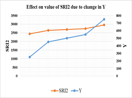
Y |
50 |
9.48 |
2948.41 |
- |
- |
|
-50 |
-9.48 |
2437.37 |
- |
- |
|
|
10 |
1.89 |
2743.99 |
- |
- |
|
|
-10 |
-1.89 |
2641.79 |
- |
- |
|
|
W |
50 |
40.63 |
3787.18 |
- |
- |
|
-50 |
-40.63 |
1598.60 |
- |
- |
|
|
10 |
8.12 |
2911.75 |
- |
- |
|
|
-10 |
-8.12 |
2474.03 |
- |
- |
|
|
MC |
50 |
- |
- |
25 |
77975.00 |
|
-50 |
- |
- |
-25 |
46785.00 |
|
|
10 |
- |
- |
5 |
65499.00 |
|
|
-10 |
- |
- |
-5 |
59261.00 |
|
|
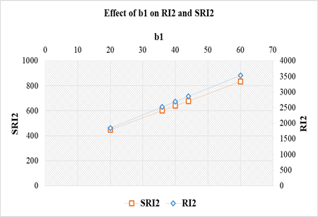
b1 |
50 |
31.23 |
3533.90 |
30.21 |
833.17 |
|
-50 |
-31.29 |
1850.21 |
-30.15 |
446.886 |
|
|
10 |
6.24 |
2861.16 |
6.04 |
678.482 |
|
|
-10 |
-6.25 |
2524.56 |
-6.03 |
601.199 |
|
|
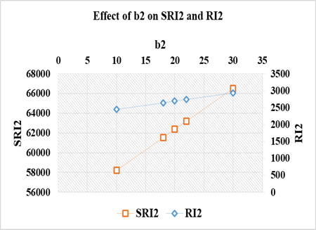
b2 |
50 |
9.19 |
2940.58 |
6.59 |
66493.20 |
|
-50 |
-9.24 |
2443.91 |
-6.62 |
58245.10 |
|
|
10 |
1.84 |
2742.52 |
1.32 |
63204.20 |
|
|
-10 |
-1.84 |
2643.21 |
-1.32 |
61555.00 |
|
|
LC |
50 |
- |
- |
25 |
77975.00 |
|
-50 |
- |
- |
-25 |
46785.00 |
|
|
10 |
- |
- |
5 |
65499.00 |
|
|
-10 |
- |
- |
-5 |
59261.00 |
|
|
c |
50 |
- |
- |
40.62 |
899.75 |
|
-50 |
- |
- |
-40.62 |
379.917 |
|
|
10 |
- |
- |
8.12 |
691.817 |
|
|
-10 |
- |
- |
8.12 |
587.85 |
Figure 4. Graphical representation of Table 2
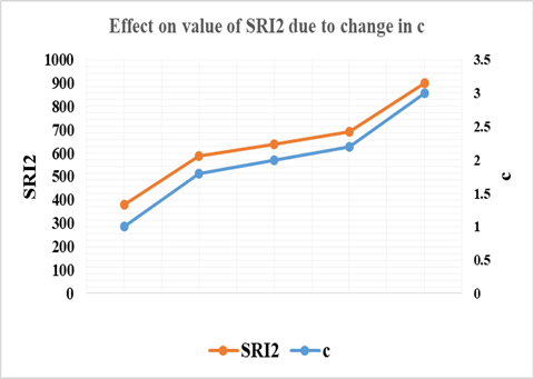
Figure 5. Effect on value of SRI2 due to change in c
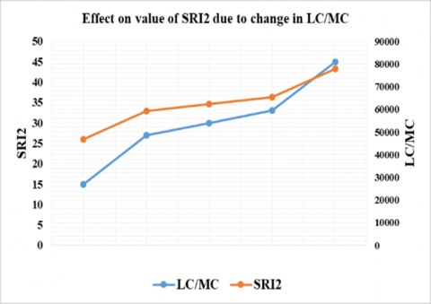
Figure 6. Effect on value of SRI2 due to change in LC/MC
Figure 7. Effect on value of RI2 due to change in Y
Figure 8. Effect on value of RI2 and SRI2 due to change in b2
Figure 9. Effect on value of RI2 due to change in W
Figure 10. Effect on value of RI2 and SRI2 due to change in b1
Under this specific segment in Table 6, we have made a comparison with the pre-existing literature [5], and the findings are that if we take the inflation as constant (same as in the research [5]), in our model, we get the reduced total cost of the retailer. And we took a variable inflation rate with a linear rise in inflation in each replenishment cycle, and the cost of the retailer increases. It thus implies that the because of variable rise in inflation the total inventory cost rises and so retailer needs more funds to bear the increased cost and thus they increase the cost of the product as well. This increased cost is then bought to equipoise by following Case 2 of the present model.
Table 6. Comparison between our model and existing literature
|
Geetha and Udayakumar [5] |
k 100 |
W - |
c 0.75 |
h 0.155 |
R 0.2 |
a 500 |
b 0.5 |
TC 1423.30 |
|
Present paper inflation constant |
Y 100 |
W 3 |
c 0.75 |
h 0.155 |
$\alpha$ 0.2 |
b1 500 |
b2 0.5 |
TC 1387.85 |
|
Present paper inflation variable |
Y 100 |
W 3 |
c 0.75 |
h 0.155 |
Variable Linear rise in inflation |
b1 500 |
b2 0.5 |
TC 1874.22 |
Our research carefully studies the market changes caused by inflation. It’s observed that inflation changes randomly so we can't keep inflation the same during the whole time frame of the model. Keeping this vibrant nature of inflation as the kernel of our research we created this near-to-market reality model. A linear rise in inflation in each replenishment cycle, results in harnessing every minute swing in inflation.
Thereafter calculating the values of the total cost of four different retailers (as shown in Table 2, by applying Algorithm 1), we used Algorithm 2, to calculate equipoise. Equipoise of the inventory cost of the retailers is calculated in coordination with the supplier. After attaining the equipoise in the cost of a product, the profits will automatically flow towards the retailers in the form of new equipoise cost (if equipoise cost is greater than the earlier cost), if the case is reversed, the supplier will offer a credit period to the remaining retailers. In this way, the supplier too will gain as he/she will now allow credit terms to the limited retailers only.
The theorem to prove that the layout under Case 2 is tenable is mentioned. Even the layout is free from any kind of stalemate point is also demonstrated in theorem 2 with the help of Lemma 1. Theorem 3 is proved to express the optimality of the total cost of the retailer.
In the managerial stance, the new model will allow managers greater leeway in making decisions. The supplier should take necessary precautions, especially in Case 2, as he/she will be solely responsible for managing the equipoise. The trade-credit period has been reduced considerably and the number of retailers to whom it will be given is also reduced, a profitable affair for suppliers furthermore.
The inventory model of equipoise is overriding all the factors which were affecting the inventory cost of the different retailers in the nabe environment to be towering high than each other. The equipoise cost will be a beneficial game for the consumer as well. Concluding we can affirm that the equipoise concept is profitable for all the contenders in the market.
For the prospects for future research, we propose the following pointers.
(i). Shortages can be incorporated and partially backlogged.
(ii). Extension can be done taking into consideration fuzzy demand.
(iii). Case 2, can be expanded for multiple suppliers-multiple retailers.
|
k |
constant, inventory dependent demand rate |
|
b1 |
increasing demand rate per year |
|
b2 |
the scaling for inflation function |
|
αi |
variable rate of inflation |
|
αi+1 |
αi+0.1 (linear rise in inflation) |
|
Y |
ordering cost per cycle |
|
W |
wholesale price per cycle |
|
h |
holding cost per cycle |
|
LC |
Labour Cost |
|
MC |
Machinery Cost |
|
c |
purchasing cost per unit (for the supplier) |
|
Ii+1 |
inventory level during (i+1) th cycle at the time ti and $t_i \leq t \leq t_{i+1}$ |
|
Qi+1 |
order quantity in (i+1) th cycle in time ti without coordination where i = 0, 1, 2,….., n-1 |
|
$S_I$ |
total cost of the supplier |
|
$M_i$ |
the tenable layout for case 2, where $i=$ $1,2,3,4, \ldots \ldots$ |
|
$C_{R_i}, i=1,2,3, \ldots$ |
the retailer who makes a proffer to the other retailer in the nabe as per Case 2 |
|
$C_i, i=1,2,3, \ldots .$. |
is the inventory cost for 10 units of the product for each retailer (used to attain equipoise in the market) |
|
$R_{I 1}$ |
total cost of first retailer |
|
$R_{I 2}$ |
total cost of second retailer |
|
$R_{I 3}$ |
total cost of third retailer |
|
$R_{I 4}$ |
total cost of fourth retailer |
|
$Q_I$ |
optimal order quantity of the system |
Appendix A
Solution of Eq. (1).
Solution will be given as:
$\begin{aligned} & \int_{t_i}^{t_{i+1}} I_{i+1}(t) e^{k t} d t=-\int_t^{t_{i+1}} e^{k u}\left(b_1 u+b_2 e^{\alpha_i u}\right) d u \\ & \int_{t_i}^{t_{i+1}} I_{i+1}(t) d t=-e^{-k t} \int_t^{t_{i+1}} e^{k u}\left(b_1 u+b_2 e^{\alpha_i u}\right) d u \\ & I_{i+1}\left(t_{i+1}\right)-I_{i+1}(t)=-e^{-k t} \int_t^{t_{i+1}}\left(b_1 u+b_2 e^{\alpha_i u}\right) d u \\ & \text { Now, } I_{i+1}\left(t_{i+1}\right)=0, \text { thus, } I_{i+1}(t)=e^{-k t} \int_t^{t_{i+1}}\left(b_1 u+b_2 e^{\alpha_i u}\right) d u \\ & t_i \leq t \leq t_{i+1}\end{aligned}$
Appendix B
Solution of Eq. (4)
Ordering cost for first cycle $=Y e^{\alpha_1\left(t_1-t_0\right)}$
Ordering cost for second cycle $=Y e^{\alpha_1\left(t_1-t_0\right)+\alpha_2\left(t_2-t_1\right)}$
Ordering cost for first and second cycle $=Y\left(e^{\alpha_1\left(t_1-t_0\right)}+\right.$ $\left.e^{\alpha_1\left(t_1-t_0\right)+\alpha_2\left(t_2-t_1\right)}\right)$
Similarly total ordering $\operatorname{cost}=Y\left(\sum_{j=0}^{n-1}\left(\left(e^{\sum_{i=0}^j \alpha_{i+1}\left(t_{i+1}-t_i\right)}\right)\right)\right)$
Appendix C
Solution of Eq. (5)
Total holding cost $=\sum_{i=0}^{n-1} h * e^{\alpha_{i+1}\left(t_{i+1}-t_1\right)} \int_{t_i}^{t_{i+1}} I_{i+1}(t) d t$
$\begin{aligned} &= \sum_{j=0}^{n-1} h * e^{\sum_{i=0}^j \alpha_{i+1}\left(t_{i+1}-t_i\right)} \int_{t_i}^{t_{i+1}} e^{-k t}\left(\int_t^{t_{i+1}} e^{k u}\left(b_1 u\right.\right. \left.\left.+b_2 e^{\alpha_i u}\right) d u\right) d t \\ &=\sum_{j=0}^{n-1} h * e^{\sum_{i=0}^j \alpha_{i+1}\left(t_{i+1}-t_i\right)} \int_{t_i}^{t_{i+1}}\left(\left(\frac{b_1}{k}\left(t_{i+1} e^{k\left(t_{i+1}-t\right)}\right.\right.\right. \left.-\frac{e^{k\left(t_{i+1}-t\right)}}{k}-t+\frac{1}{k}\right) \\ &+\left(\frac{b_2}{\alpha_{i+1}+k}\left(e^{\alpha_{i+1} t_{i+1} * e^{k\left(t_{i+1}-t\right)}}\right.\right. \left.\left.-e^{\alpha_{i+1}\, t}\right)\right) d t \sum_{j=0}^{n-1} h * e^{\sum_{i=0}^j \alpha_{i+1}\left(t_{i+1}-t_i\right)}\left(\frac{b_1 t_{i+1}}{k} \int_{t_i}^{t_{i+1}} e^{k\left(t_{i+1}-t\right)} d t\right. -\frac{b_1}{k^2} \int_{t_i}^{t_{i+1}} e^{k\left(t_{i+1}-t\right)} d t \\ &+\frac{b_1}{k} \int_{t_i}^{t_{i+1}}\left(-t+\frac{1}{k}\right) d t +\frac{b_2 e^{\alpha_{i+1} t_{i+1}}}{\alpha_{i+1}+k} \int_{t_i}^{t_{i+1}} e^{k\left(t_{i+1}-t\right)} d t \left.-\frac{b_2}{\alpha_{i+1}+k} \int_{t_i}^{t_{i+1}} e^{\alpha_{i+1}\,\, t} d t\right)\end{aligned}$
$\begin{aligned} &=\sum_{j=0}^{n-1} h * e^{\sum_{i=0}^j \alpha_{i+1}\left(t_{i+1}-t_i\right)}\left(\left(-\frac{b_1 * t_{i+1}}{k^2}\left(1-e^{k\left(t_{i+1}-t_i\right)}\right)+\frac{b_1}{k^3}(1\right.\right. \left.-e^{k\left(t_{i+1}-t_i\right)}\right)+\frac{b_1}{k^2}\left(t_{i+1}-t_i\right)-\frac{b_1}{2 k}\left(t_{i+1}^2-t_i^2\right) \\ & -\frac{b_2 * e^{\alpha_{i+1}\,\, t_{i+1}}}{k\left(\alpha_{i+1}+k\right)}\left(1-e^{k\left(t_{i+1}-t_i\right)}\right) \left.-\frac{b_2 * e^{\alpha_{i+1}\left(t_{i+1}-t_i\right)}}{\alpha_{i+1}\left(\alpha_{i+1}+k\right)}\right) \\ & h\left(\sum_{j=0}^{n-1}\left(\left(e^{\sum_{i=0}^j \alpha_{i+1}\left(t_{i+1}-t_i\right)}\right) * \frac{1}{2 k^3} b_1\left(2-2 e^{k\left(-t_j+t_{1+j}\right)}-2 k t_j\right.\right.\right. \\ & \left.+k^2 t_j^2+2 e^{k\left(-t_j+t_{1+j}\,\,\right)} k t_{1+j}-k^2 t_{1+j}^2\right) \left.+\frac{b_2\left(\frac{e^{-k t_j+t_{1+j} \alpha_\,{1+j}\left(-e^{k t_j}+e^{k t_{1+j}}\right)}}{k}+\frac{e^{t_j \alpha_{1+j}}-e^{t_{1+j} \alpha_{1+j}}}{\alpha_{1+j}}\right)}{k+\alpha_{1+j}}\right) \\ & \end{aligned}$
Appendix D
Solution of Eq. (6)
Total purchasing cost $=W\left(\sum_{j=0}^{n-1}\left(\left(e^{\sum_{i=0}^j \alpha_{i+1}\left(t_{i+1}-t_i\right)}\right) * Q_{j+1}\right.\right.$
$\begin{aligned} \text { where } Q_{j+1}=e^{-k t_j} & \int_{t_j}^{t_{j+1}} e^{k t}\left(b_1 t+b_2 e^{\alpha_{j+1} t}\right) d t =W\left(\sum_{j=0}^{n-1}\left(\left(e^{\sum_{i=0}^j \alpha_{i+1}\left(t_{i+1}-t_i\right)}\right)\right.\right. *\left(e^{-k t_j}\left(\int_{t_j}^{t_{j+1}} e^{k t} b_1 t d t\right.\right. \left.\left.+\int_{t_j}^{t_{j+1}} b_2 e^{\left(\alpha_{j+1}+k\right) t} d t\right)\right) \\ &=W\left(\sum_{j=0}^{n-1}\left(\left(e^{\sum_{i=0}^j \alpha_{i+1}\left(t_{i+1}-t_i\right)}\right)\right.\right. *\left(\left(b_1\left(\frac{e^{k\left(t_{j+1}-t_j\right)} * t_{j+1}}{k}-\frac{e^{k\left(t_{j+1}-t_j\right)}}{k^2}-\frac{t_j}{k}+\frac{1}{k^2}\right)\right.\right. \\ & +b_2\left(\frac{\left.\left.\left.e^{\alpha_{j+1} * t_{j+1} * e^{k\left(t_{j+1}-t_j\right)}-e^{t_{j *} * \alpha_{j+1}}}\right)\right)\right)}{k+\alpha_{j+1}}\right)\end{aligned}$
Appendix E
Proof of Theorem 1: In-depth analysis of Figure 2, indicates that there will be no circulation proffer offered by any retailer as the proffer will travel from highest to lowest inventory cost.
Let’s suppose that, the layout is untenable, thus, there will be a set of two nabe retailers, $C_{R_m}\left(t_i\right)$ and $C_{R_n}\left(t_i\right), m, n \in$$M_i$ s.t. $C_{R_m}$, is the retailer having the largest value of inventory cost in the nabe and $C_{R_n}\left(t_i\right)$, is the retailer having the lowest inventory cost in the nabe. Moreover, $C_m-C_n$ is the highest inventory cost difference in the nabe. Following this, the retailer $C_{R_m}\left(t_i\right)$ will make a proffer to $C_{R_n}\left(t_i\right)$ and $C_{R_n}\left(t_i\right)$ will accept the proffer, resulting in CostPact between $C_{R_m}\left(t_i\right)$ and $C_{R_n}\left(t_i\right)$ . Since, $C_{R_n}\left(t_i\right)$ is increased at the time $t_{i+1}, n \in M_i$ holds.
Appendix F
Proof of Theorem 2
According to Lemma 1, $D\left(t_i\right)>D\left(t_{i+1}\right)$, this implies, that eventually, the differences among the inventory costs are reducing with every proffer made.
Moreover, theorem 1, proves that there is no stalemate point in the layout $M_i$, thus the layout will reach equipoise. (As the value of k increases, the equipoise is attained in lesser loops). (Refer to Algorithm 2 for equipoise).
Lemma 1: Let $D\left(t_i\right)=\operatorname{high}_{i \in M_i} C_i\left(t_i\right)-\operatorname{low}_{i \in M_i} C_i\left(t_i\right)$. As long as $C_i\left(t_i\right) \neq \phi$, we have $D\left(t_i\right)>D\left(t_{i+1}\right)$
Proof: To start with, let us consider, $i \notin M_i$. Since retailer, $R_i$ does not pass a proffer to any other retailer in the layout, there will be no change in its inventory cost. Thus, $\operatorname{high}_{i \in M_i}\left[\frac{C_i\left(t_i\right)-C_j\left(t_i\right)}{k}\right]=0$ holds.
Now, suppose that a retailer has the highest inventory cost in $M_i$. As no nabe retailer will make a proffer to such a retailer, the cost will be down at the time $t_{i+1}$. If a retailer has the lowest inventory cost in $M_i$, the nabe retailer will make a proffer to such retailer. Thus, the inventory cost will rise at the time $t_{i+1}$. Suppose, $C_i^{\text {high2 }}\left(t_i\right)$ be the second highest inventory cost among all the retailers in the layout. Then, the cost will not exceed $C_i^{h i g h 2}\left(t_i\right)$ at time $t_{i+1}$ as it will go up only when it accepts a proffer made by only such retailer which has higher inventory cost than $C_i^{\text {high2 }}\left(t_i\right)$. Even if this scenario takes place, the increment in the inventory cost will be at the maximum, half (taking $\mathrm{k}=2$ ), of the difference between the inventory costs. Thus, we have, $C_i^{h i g h}\left(t_i\right)>$ $C_i^{\text {high2 }}\left(t_{i+1}\right)$ and $C_i^{\text {high }}\left(t_i\right)>C_i^{\text {high }}\left(t_{i+1}\right)$.
On the other side, the retailer $C_i^{\text {low }}\left(t_i\right)$ will accept the proffer and its inventory cost will raise at the time $\left(t_{i+1}\right)$ Suppose, $C_i^{\text {low2 }}\left(t_i\right)$ is the second lowest inventory cost among all the retailers in the layout. Then, it will at the maximum, decrease without any proffer only when it is in contact with such a retailer which have $C_i^{\text {low }}\left(t_i\right)$. Thus, we have, $C_i^{\text {low }}\left(t_i\right) \leq C_i^{\text {low } 2}\left(t_{i+1}\right)$, and $C_i^{\text {low }}\left(t_i\right) \leq C_i^{\text {low }}\left(t_{i+1}\right)$.
As a result, $D\left(t_j\right)>D\left(t_{i+1}\right)$ holds true.
Appendix G
Proof of Theorem 3:
Proof: We will find out the following first and second-order derivatives:
$\begin{aligned} & \frac{\partial R_{I 2}}{\partial t_i}=h\left\{\left(\alpha_i-\alpha_{1+i}\right) *\left(e^{\sum_{i=0}^j \alpha_{i+1}\left(t_{i+1}-t_i\right)}\right) *\left(\frac{1}{2 k^3} b_1(2-\right.\right. 2 e^{k\left(-t_j+t_{1+j}\right)}\\&-2 k t_j+k^2 t_j^2+2 e^{k\left(-t_j+t_{1+j}\right)} k t_{1+j}- \left.\left.k^2 t_{1+j}^2\right)+\frac{b_2\left(\frac{e^{-k t_j+t_{1+j} \alpha_{1+j}}\left(-e^{k t_j}+e^{k t_{1+j}}\right)}{k}+\frac{e^{t_j \alpha_{1+j}} e_{-e^{t_{1+j} \alpha_{1+j}}}}{\alpha_{1+j}}\right)}{k+\alpha_{1+j}}\right)+\end{aligned}$
$\begin{aligned} & \left(e^{\sum_{i=0}^j \alpha_{i+1}\left(t_{i+1}-t_i\right)}\right) * \frac{\left(-e^{k\left(-t_{-1+i}+t_i\right)} k+e^{k\left(-t_i+t_{1+i}\right)} k\right) b_1}{k^3}+ \frac{b_1\left(-1+e^{k\left(-t_{-1+i}+t_i\right)}+e^{k\left(-t_{-1+i}+t_i\right)} k t_i-e^{\left.k\left(-t_i+t_{1+i}\right)_k t_{1+i}\right)}\right.}{k^2}+ \\ & \frac{e^{k\left(-t_{-1+i}+t_i\right)+t_i \alpha_i} b_2}{k+\alpha_i}+\frac{e^{t_i \alpha_{i b_2}\left(-\frac{1}{k}+\frac{e^{k\left(-t_{-1+i}+t_i\right)}}{k}-\frac{1}{\alpha_i}\right) \alpha_i}}{k+\alpha_i}+\frac{e^{t_i \alpha_{1+i} b_2}}{k+\alpha_{1+i}}-\end{aligned}$
$\begin{aligned} & \left.\frac{e^{k\left(-t_i+t_{1+i}\right)+t_{1+i} \alpha_{1+i} b_2}}{k+\alpha_{1+i}}\right\}+Y\left\{e^{\sum_{i=0}^{i-1} \alpha_{i+1}\left(t_{i+1}-t_i\right)} *\left(\alpha_i-\right.\right. \left.\left.\alpha_{i+1}\right)\right\}+e^{\sum_{i=0}^i \alpha_{i+1}\left(t_{i+1}-t_i\right)} *\left(\alpha_i-\alpha_{i+1}\right) * \\ & \left(b_1\left(\frac{e^{k\left(t_{i+1}-t_i\right)_* t_{i+1}}}{k}-\frac{e^{k\left(t_{i+1}-t_i\right)}}{k^2}-\frac{t_i}{k}+\frac{1}{k^2}\right)+\right. \left.b_2\left(\frac{e^{\alpha_{i+1} * t_{i+1 *} * e^{k\left(t_{i+1}-t_i\right)}-e^{t_i^* \alpha_{i+1}}}}{k+\alpha_{i+1}}\right)\right)+e^{\sum_{i=0}^i \alpha_{i+1}\left(t_{i+1}-t_i\right)} * \\ & \left(b_1\left(-\frac{1}{k}+\frac{e^{k\left(-t_i+t_{1+i}\right)}}{k}-e^{k\left(-t_i+t_{1+i}\right)} * t_{1+i}\right)+\right. \left.\left.\frac{\left.\left.b_2\left(-e^{k\left(-t_i+t_{1+i}\right)+t_{1+i}^* \alpha_{1+i} k-e^{\left.t_i^* \alpha_{1+i} \alpha_{1+i}\right)}}\right)\right)\right\}}{k+\alpha_{1+i}}\right)\right\} \\ & \end{aligned}$
$\begin{aligned} & \frac{\partial^2 R_{I 2}}{\partial t_i^2}=\frac{e^{\left(-t_i+t_{1+i}\right) \alpha_{1+i}}\, h b_1\left(2 k^2-2 e^{k\left(-t_i+t_{1+i}\right)} k^2+2 e^{k\left(-t_i+t_{1+i}\right)} k^3 t_{1+i}\right)}{2 k^3}-\frac{e^{\left(-t_i+t_{1+i}\right) \alpha_{1+i}} h b_1}{k^3} * \frac{\left(-2 k+2 e^{k\left(-t_i+t_{1+i}\right)} k+2 k^2 t_i-2 e^{k\left(-t_i+t_{1+i}\right)} k^2 t_{1+i}\right) \alpha_{1+i}}{k^3}+\\ &e^{\left(-t_i+t_{1+i}\right) \alpha_{1+i}} Y \alpha_{1+i}^2 +e^{\left(-t_i+t_{1+i}\right) \alpha_{1+i}} \alpha_{1+i}^2\left(b_1\left(\frac{1}{k^2}-\frac{e^{k\left(-t_i+t_{1+i}\right)}}{k^2}-\frac{t_i}{k}+\frac{e^{k\left(-t_i+t_{1+i}\right)} t_{1+i}}{k}\right)+\frac{\left(-e^{t_i \alpha_{1+i}}+e^{\left.k\left(-t_i+t_{1+i}\right)+t_{1+i} \alpha_{1+i}\right) b_2}\right)}{k+\alpha_{1+i}}\right) +e^{\left(-t_i+t_{1+i}\right) \alpha_{1+i}} h \alpha_{1+i}^2 \\ &*\left(\frac{b_1\left(2-2 e^{k\left(-t_i+t_{1+i}\right)}-2 k t_i+k^2 t_i^2+2 e^{k\left(-t_i+t_{1+i}\right)} k t_{1+i}-k^2 t_{1+i}^2\right)}{2 k^3}\right. \left.+\frac{e^{\mathrm{kt}_i+t_{1+i} \alpha_{1+i}}\left(-e^{\mathrm{kt}_i}+e^{\mathrm{kt}_{1+i}}\right) b_2}{k\left(k+\alpha_{1+i}\right)}\right)-2 e^{\left(-t_i+t_{1+i}\right) \alpha_{1+i}} \alpha_{1+i}\left(b_1\left(-\frac{1}{k}+\frac{e^{k\left(-t_i+t_{1+i}\right)}}{k}-e^{k\left(-t_i+t_{1+i}\right)} t_{1+i}\right)\right. \\ & \left.+\frac{b_2\left(-e^{k\left(-t_i+t_{1+i}\right)+t_{1+i} \alpha_{1+i}} k-e^{t_i \alpha_{1+i}} \alpha_{1+i}\right)}{k+\alpha_{1+i}}\right)+e^{\left(-t_i+t_{1+i}\right) \alpha_{1+i}}\left(b_1\left(-e^{k\left(-t_i+t_{1+i}\right)}+e^{k\left(-t_i+t_{1+i}\right)} k t_{1+i}\right)\right. \left.+\frac{b_2\left(e^{k\left(-t_i+t_{1+i}\right)+t_{1+i} \alpha_{1+i}} k^2-e^{t_i \alpha_{1+i}} \alpha_{1+i}^2\right)}{k+\alpha_{1+i}}\right) \\ & \end{aligned}$
$\begin{aligned} & \frac{\partial^2 R_{I 2}}{\partial t_i \partial t_{i+1}}=-e^{k\left(-t_i+t_{1+i}\right)+\left(-t_i+t_{1+i}\right) \alpha_{1+i}} h b_1 t_{1+i}+e^{\left(-t_i+t_{1+i}\right) \alpha_{1+i}}\left(-e^{k\left(-t_i+t_{1+i}\right)+t_{1+i} \alpha_{1+i}} k b_2-e^{k\left(-t_i+t_{1+i}\right)} k b_1 t_{1+i}\right) +\frac{e^{\left(-t_i+t_{1+i}\right) \alpha_{1+i}} h b_1}{2 k^3} \\ &* \frac{\left(-2 k+2 e^{k\left(-t_i+t_{1+i}\right)} k+2 k^2 t_i-2 e^{k\left(-t_i+t_{1+i}\right)} k^2 t_{1+i}\right) \alpha_{1+i}}{2 k^3} -e^{\left(-t_i+t_{1+i}\right) \alpha_{1+i}}\left(e^{k\left(-t_i+t_{1+i}\right)+t_{1+i} \alpha_{1+i}} b_2+e^{k\left(-t_i+t_{1+i}\right)} b_1 t_{1+i}\right) \alpha_{1+i}-e^{\left(-t_i+t_{1+i}\right) \alpha_{1+i}} Y \alpha_{1+i}^2 \\ & -e^{\left(-t_i+t_{1+i}\right) \alpha_{1+i}} \alpha_{1+i}^2\left(b_1\left(\frac{1}{k^2}-\frac{e^{k\left(-t_i+t_{1+i}\right)}}{k^2}-\frac{t_i}{k}+\frac{e^{k\left(-t_i+t_{1+i}\right)} t_{1+i}}{k}\right)+\frac{\left(-e^{t_i \alpha_{1+i}}+e^{\left.k\left(-t_i+t_{1+i}\right)+t_{1+i} \alpha_{1+i}\right) b_2}\right.}{k+\alpha_{1+i}}\right) -\frac{e^{\left(-t_i+t_{1+i}\right) \alpha_{1+i}} h \alpha_{1+i}^2}{2 k^3} \\ &*\left(\frac{b_1\left(2-2 e^{k\left(-t_i+t_{1+i}\right)}-2 k t_i+k^2 t_i^2+2 e^{k\left(-t_i+t_{1+i}\right)} k t_{1+i}-k^2 t_{1+i}^2\right)}{2 k^3}\right. \left.+\frac{e^{\mathrm{kt}_i+t_{1+i} \alpha_{1+i}}\left(-e^{\mathrm{kt}_i}+e^{\mathrm{kt}_{1+i}}\right) b_2}{k\left(k+\alpha_{1+i}\right)}\right)-e^{\left(-t_i+t_{1+i}\right) \alpha_{1+i}} h \alpha_{1+i}\left(\frac{b_1\left(-2 k^2 t_{1+i}+2 e^{k\left(-t_i+t_{1+i}\right)} k^2 t_{1+i}\right)}{2 k^3}\right. \\ & \left.+\frac{e^{\mathrm{kt}_i+t_{1+i} \alpha_{1+i}}\left(-e^{\mathrm{kt}_i}+e^{\mathrm{kt}_{1+i}}\right) b_2 \alpha_{1+i}}{k\left(k+\alpha_{1+i}\right)}\right)+e^{\left(-t_i+t_{1+i}\right) \alpha_{1+i}} \alpha_{1+i}\left(b_1\left(-\frac{1}{k}+\frac{e^{k\left(-t_i+t_{1+i}\right)}}{k}-e^{k\left(-t_i+t_{1+i}\right)} t_{1+i}\right)\right. \left.+\frac{b_2\left(-e^{k\left(-t_i+t_{1+i}\right)+t_{1+i} \alpha_{1+i}} k-e^{t_i \alpha_{1+i}} \alpha_{1+i}\right)}{k+\alpha_{1+i}}\right) \\ & \end{aligned}$
$\begin{aligned} & \frac{\partial^2 R_{I 2}}{\partial t_i \partial t_{i-1}}=-e^{k\left(-t_{-1+i}+t_i\right)+\left(-t_{-1+i}+t_i\right) \alpha_i} h b_1 t_i+e^{\left(-t_{-1+i}+t_i\right) \alpha_i}\left(-e^{k\left(-t_{-1+i}+t_i\right)+t_i \alpha_i} k b_2-e^{k\left(-t_{-1+i}+t_i\right)} k b_1 t_i\right)+\frac{e^{\left(-t_{-1+i}+t_i\right) \alpha_i} h b_1}{2 k^3} * \frac{\left(-2 k+2 e^{k\left(-t_{-1+i}+t_i\right)} k-2 e^{k\left(-t_{-1+i}+t_i\right)} k^2 t_i\right) \alpha_i}{2 k^3}\\ &-e^{\left(-t_{-1+i}+t_i\right) \alpha_i}\left(e^{k\left(-t_{-1+i}+t_i\right)+t_i \alpha_i} b_2+e^{k\left(-t_{-1+i}+t_i\right)} b_1 t_i\right) \alpha_i -e^{\left(-t_{-1+i}+t_i\right) \alpha_i} Y \alpha_i^2-e^{\left(-t_{-1+i}+t_i\right) \alpha_i} \alpha_i^2\left(b_1\left(\frac{1}{k^2}-\frac{e^{k\left(-t_{-1+i}+t_i\right)}}{k^2}-\frac{t_{-1+i}}{k}+\frac{e^{k\left(-t_{-1+i}+t_i\right)} t_i}{k}\right)\right. \\ & \left.+\frac{\left(-e^{t_{-1+i} \alpha_i}+e^{k\left(-t_{-1+i}+t_i\right)+t_i \alpha_i}\right) b_2}{k+\alpha_i}\right)-\frac{e^{\left(-t_{-1+i}+t_i\right) \alpha_i} h \alpha_i^2}{2 k^3} *\left(\frac{b_1\left(2-2 e^{k\left(-t_{-1+i}+t_i\right)}-2 k t_{-1+i}+2 e^{k\left(-t_{-1+i}+t_i\right)} k t_i\right)}{2 k^3}+\frac{e^{\mathrm{kt}_i+t_i \alpha_i}\left(-e^{\mathrm{kt}_i}+e^{\left.\mathrm{kt}_{1+i}\right)}\right) b_2}{k\left(k+\alpha_i\right)}\right) \\ & -e^{\left(-t_{-1+i}+t_i\right) \alpha_i} h \alpha_i\left(\frac{e^{k\left(-t_{-1+i}+t_i\right)} b_1 t_i}{k}+\frac{e^{\mathrm{kt}_i+t_i \alpha_i}\left(-e^{\mathrm{kt}_i}+e^{\mathrm{kt}_{1+i}}\right) b_2 \alpha_i}{k\left(k+\alpha_i\right)}\right)+e^{\left(-t_{-1+i}+t_i\right) \alpha_i} \alpha_i\left(b_1\left(-\frac{1}{k}\right.\right. \left.\left.+\frac{e^{k\left(-t_{-1+i}+t_i\right)}}{k}-e^{k\left(-t_{-1+i}+t_i\right)} t_i\right)+\frac{b_2\left(-e^{k\left(-t_{-1+i}+t_i\right)+t_i \alpha_i} k-e^{t_{-1+i} \alpha_i} \alpha_i\right)}{k+\alpha_i}\right) \\ & \end{aligned}$$\frac{\partial^2 R_{I 2}}{\partial t_i \partial t_k}=0 \text { for all } k \neq i-1, i, i+1$
Moreover,
$\frac{\partial^2 R_{I 2}}{\partial t_i^2}>\left|\frac{\partial^2 R_{I 2}}{\partial t_i t_{i-1}}\right|+\left|\frac{\partial^2 R_{I 2}}{\partial t_i t_{i+1}}\right|, \forall i=1,2,3, \ldots \ldots, n-1$
Thus, the Hessian matrix will be a diagonal matrix and all the diagonal elements will be positive and it will be positive definite.
$\nabla^2 R_{I 2}=\left(\begin{array}{ccccccccc}\frac{\partial^2 R_{12}}{\partial t_1^2} & \frac{\partial^2 R_{12}}{\partial t_1 \partial t_2} & 0 & 0 & 0 & 0 & 0 & 0 & 0 \\ \frac{\partial^2 R_{12}}{\partial t_2 t_1} & \frac{\partial^2 R_{12}}{\partial t_2^2} & \frac{\partial^2 R_{12}}{\partial t_2 \partial t_3} & 0 & 0 & 0 & 0 & 0 & 0 \\ 0 & \frac{\partial^2 R_{12}}{\partial t_{32} t_2} & \frac{\partial^2 R_{12}}{\partial t_3^2} & \frac{\partial^2 R_{12}}{\partial t_3 \partial_4} & 0 & 0 & 0 & 0 & 0 \\ \ldots & \ldots & \ldots & \ldots & \ldots & \ldots & \ldots & \ldots & \ldots \\ 0 & 0 & 0 & 0 & 0 & 0 & 0 & 0 & 0 \\ 0 & 0 & 0 & 0 & 0 & 0 & \frac{\partial^2 R_{12}}{\partial t_{n-1} \partial t_{n-2}} & \frac{\partial^2 R_{12}}{\partial t_{n-1}^2} & \frac{\partial^2 R_{12}}{\partial t_{n-1} \partial t_n} \\ 0 & 0 & 0 & 0 & 0 & 0 & 0 & \frac{\partial^2 R_{12}}{\partial t_n \partial t_{n-1}} & \frac{\partial^2 R_{12}}{\partial t_n^2}\end{array}\right)$
Thus, the Eq. (10), will have unique solution with the global minimum and the unique solution is the optimal replenishment cycle length.
[1] Buzacott, J.A. (1975). Economic order quantities with inflation. Journal of the Operational Research Society, 26(3): 553-558. https://doi.org/10.1057/jors.1975.113
[2] Guria, A., Das, B., Mondal, S. Maiti, M. (2013). Inventory policy for an item with inflation induced purchasing price, selling price and demand with immediate part payment. Applied Mathematical Modelling, 37(1-2): 240-257. https://doi.org/10.1016/j.apm.2012.02.010
[3] Goyal, S.K. (1985). Economic order quantity under conditions of permissible delay in payments. Journal of Operations Research Society, 36(4): 335-338. https://doi.org/10.2307/2582421
[4] Aggarwal, S.P., Jaggi, C.K. (1995). Ordering policies of deteriorating items under permissible delay in payments. Journal of the Operational Research Society, 46(5): 658-662. https://doi.org/10.1057/jors.1995.90
[5] Esmaeili, M., Nasrabadi, M. (2020). An inventory model for single-vendor multi-retailer supply chain under inflationary conditions and trade credit. Journal of Industrial and Production Engineering, 38(2):75-88. https://doi.org/10.1080/21681015.2020.1845248
[6] Mirzazadeh, A., Seyyed Esfahani, M.M., Fatemi Ghomi, S.M.T. (2009). An inventory model under uncertain inflationary conditions, finite production rate and inflation-dependent demand rate for deteriorating items with shortages. International Journal of Systems Science, 40(1): 21-31. https://doi.org/10.1080/00207720802088264
[7] Tripathi, R.P. (2011). Optimal pricing and ordering policy for inflation dependent demand rate under permissible delay in payments. International Journal of Business, Management and Social Sciences, 2(4): 35-43.
[8] Shastri, A., Singh, S.R., Yadav, D., Gupta, S. (2013). Multi-echelon supply chain management for deteriorating items with partial backordering under inflationary environment. Procedia Technology, 10: 320-329. https://doi.org/10.1016/j.protcy.2013.12.367
[9] Singh, S.P., Panda, G.C. (2015). An inventory model for generalized weibull deteriorating items with price dependent demand and permissible delay in payments under inflation. LogForum, 11(3): 259-266. https://doi.org/10.17270/J.LOG.2015.3.5
[10] Kiniwa, J., Kikuta, K., Sandoh, H. (2015). An inflation/deflation model for price stabilization in networks. In ICAART, (1): 125-132. https://doi.org/10.5220/0005186101250132
[11] Geetha, K.V., Udayakumar, R. (2020). Economic ordering policy for deteriorating items with inflation induced time dependent demand under infinite time horizon. International Journal of Operational Research, 39(1): 69-94. https://doi.org/10.1504/IJOR.2020.108835
[12] Sundararajan, R., Vaithyasubramanian, S., Nagarajan, A. (2020). Impact of delay in payment, shortage and inflation on an EOQ model with bivariate demand. Journal of Management Analytics, 8(2): 267-294. https://doi.org/10.1080/23270012.2020.1811165
[13] Sundararajan, R., Vaithyasubramanian, S., Rajinikannan, M. (2021). Price determination of a non-instantaneous deteriorating EOQ model with shortage and inflation under delay in payment. International Journal of Systems Science: Operations & Logistics, 9(3): 384-404. https://doi.org/10.1080/23302674.2021.1905908
[14] Chung, K.J., Liao, J.J., Ting, P.S., Lin, S.D., Srivastava, H.M. (2018). A unified presentation of inventory models under quantity discounts, trade credits and cash discounts in the supply chain management. Revista de la Real Academia de Ciencias Exactas, Físicas y Naturales. Serie A. Matemáticas, 112: 509-538. https://doi.org/10.1007/s13398-017-0394-7
[15] Zhong, Y.G., Shu, J., Xie, W., Zhou, Y.W. (2018). Optimal trade credit and replenishment policies for supply chain network design. Omega, 81: 26-37. https://doi.org/10.1016/j.omega.2017.09.006
[16] Mahato, C., De, S.K., Mahata, G.C. (2021). Joint pricing and inventory management for growing items in a supply chain under trade credit. Soft Computing, 25(11): 7271-7295. https://doi.org/10.1007/s00500-021-05635-2
[17] Mandal, B., Dey, B.K., Khanra, S., Sarkar, B. (2021). Advance sustainable inventory management through advertisement and trade-credit policy. RAIRO-Operations Research, 55(1): 261-284. https://doi.org/10.1051/ro/2020067
[18] Wu, C.F., Zhao, Q.H. (2014). Supplier–retailer inventory coordination with credit term for inventory‐dependent and linear‐trend demand. International Transactions in Operational Research, 21(5): 797-818. https://doi.org/10.1111/itor.12060
[19] Singh, P., Mishra, N.K., Singh, V., Saxena, S. (2017). An EOQ model of time quadratic and inventory dependent demand for deteriorated items with partially backlogged shortages under trade credit. In AIP Conference Proceedings, AIP Publising LLC, 1860(1): 020037. https://doi.org/10.1063/1.4990336
[20] Singh, V., Saxena, S., Gupta, R.K., Mishra, N.K., Singh, P. (2018). A supply chain model with deteriorating items under inflation. In 2018 4th International Conference on Computing Sciences, IEEE, 119-125. https://doi.org/10.1109/ICCS.2018.00028
[21] Singh, V., Mishra, N.K., Mishra, S., Singh, P., Saxena, S. (2019). A green supply chain model for time quadratic inventory dependent demand and partially backlogging with Weibull deterioration under the finite horizon. In AIP Conference Proceedings, AIP Publishing LLC, 2080(1): 060002. https://doi.org/10.1063/1.5092937
[22] Taghizadeh-Yazdi, M., Farrokhi, Z., Mohammadi-Balani, A. (2020). An integrated inventory model for multi-echelon supply chains with deteriorating items: A price-dependent demand approach. Journal of Industrial and Production Engineering, 37(2-3): 87-96. https://doi.org/10.1080/21681015.2020.1733679
[23] Liao, H.C., Tsai, C.H., Su, C.T. (2000). An inventory model with deteriorating items under inflation when a delay in payment is permissible. International Journal of Production Economics, 63(2): 207-214. https://doi.org/10.1016/S0925-5273(99)00015-8
[24] Kumar, S., Rajput, U.S. (2015). An inventory model for perishable items with time varying stock dependent demand and trade credit under inflation. American Journal of Operations Research, 5(05): 435. https://doi.org/10.4236/ajor.2015.55036
[25] Saha, S., Sen, N. (2019). An inventory model for deteriorating items with time and price dependent demand and shortages under the effect of inflation. International Journal of Mathematics in Operational Research, 14(3): 377-388. https://doi.org/10.1504/IJMOR.2019.099385
[26] Shaikh, A.A., Khan, M.A.A., Panda, G.C., Konstantaras, I. (2019). Price discount facility in an EOQ model for deteriorating items with stock‐dependent demand and partial backlogging. International Transactions in Operational Research, 26(4): 1365-1395. https://doi.org/10.1111/itor.12632
[27] Barman, H., Pervin, M., Roy, S.K., Weber, G.W. (2021). Back-ordered inventory model with inflation in a cloudy-fuzzy environment. Journal of Industrial and Management Optimization, 17(4): 1913-1941. https://doi.org/10.3934/jimo.2020052
[28] Khan, M.A.A., Shaikh, A.A., Cárdenas-Barrón, L.E., Mashud, A.H.M., Treviño-Garza, G., Céspedes-Mota, A. (2022). An inventory model for non-instantaneously deteriorating items with nonlinear stock-dependent demand, hybrid payment scheme and partially backlogged shortages. Mathematics, 10(3): 434. https://doi.org/10.3390/math10030434
[29] Nemtajela, N., Mbohwa, C. (2017). Relationship between inventory management and uncertain demand for fast moving consumer goods organisations. Procedia Manufacturing, 8: 699-706. https://doi.org/10.1016/j.promfg.2017.02.090
[30] Jaggi, C.K., Gupta, M., Kausar, A., Tiwari, S. (2019) Inventory and credit decisions for deteriorating items with displayed stock dependent demand in two-echelon supply chain using Stackelberg and Nash equilibrium solution. Annals of Operations Research, 274: 309-329. https://doi.org/10.1007/s10479-018-2925-9
[31] Li, J.B., Guan, M.C., Chen, Z.Y. (2020). Optimal inventory policy for fast-moving Consumer goods under e-commerce environment. Journal of Industrial and Management Optimization, 16(4): 1769-1781. https://doi.org/10.3934/jimo.2019028