Ichwana Ramli*![]() | Siti Rusdiana
| Siti Rusdiana![]() | Ashfa Achmad
| Ashfa Achmad![]() | Azizah
| Azizah![]() | Monisa Eka Yolanda
| Monisa Eka Yolanda![]()
© 2023 IIETA. This article is published by IIETA and is licensed under the CC BY 4.0 license (http://creativecommons.org/licenses/by/4.0/).
OPEN ACCESS
Climate change which has become increasingly erratic in recent decades has become a problem of global warming. So that it has an impact and influence in changing rainfall patterns. A very volatile climate overall can threaten the success of food production. Information about rainfall patterns is very important to agriculture that relies on rainfall as the main source of irrigation. The purpose of this study is to predict rainfall from all time series based on rainfall data for 15 years, 10 years and 5 years. Prediction results were evaluated using the Nash-Sutcliffe Efficiency (NSE) statistical method, RMSE-Observation Standard Deviation Ratio (RSR) and PBIAS. This research was conducted in Aceh Besar District. Indonesia which coincided with Indrapuri District. Analysis of the data used in this study uses the Seasonal Autoregressive Integrated Moving Average (SARIMA) models. The best prediction results are generated from the use of rainfall time series data onto 5 years for 2013-2017 with the evaluation value of the model obtained is in the “Very Good " category. Prediction models for the best rainfall predictions are (0.0.0) and (0.1.2)12 with the respective values of NSE of 0.84, RSR 0.41 and PBIAS - 2.8. So as a whole the closest prediction results in the actual values are obtained from time series rainfall data onto the past five years.
rainfall, forecasting, Seasonal Autoregressive Integrated Moving Average (SARIMA), TIME series
The increasingly uncertain climate conditions in the last few decades around the world have had an impact on the declining rainfall trend. Natural resource management is strongly driven by climate. The impact of climate change has an impact on ecology, natural resource degradation and hydrology. Rainfall characteristics are very important to know. This is because at this time there has been the instability of rainfall patterns that occur due to climate change. Climate change has caused an increase in average air temperatures [1]. The average temperature is increase from 26.77℃ to 27.3℃ in the period 1992-2002 to 2002-2011 (Peusangan watershed Aceh, Indonesia). The decrease in rainfall intensity is one of the impacts of climate change that has caused a decrease in agricultural output such as rice [2]. Therefore, information about rainfall patterns that might occur in the future is needed one way that can be done to find out rainfall information is to make predictions with all possibilities.
The relationship between the frequency and duration of rainfall intensity is a representation of the amount of water that falls in a certain period of time [3]. So that it can be used to determine the time of puddle, and when a certain level of rainfall or flow volume will recur in the future [4]. This is needed as a step in making policies. Therefore, information about rainfall patterns that may occur in the future is needed. One way that can be done to find out rainfall information is to make predictions with all possibilities.
Prediction is defined as an attempt made to predict the situation in the future by testing the situation in the past. The main value of forecasting is to make events in the past as a basis or reference for decision making by implementing various policies in the future [5-7]. Predictions can be made using time series analysis which can provide information about trends data. Prediction rainfall and discharge using vector Autoregressive has been carried out [8]. Cycles or fluctuations around the average length value, so that it can be used as a modelling and prediction tool [9-11]. The order of the values of the variables observed at certain continuous time intervals is called the time series [12]. Forecasting is done to predict future events that involve the collection of historical data that will be projected using a mathematical model [13].
The time series method is able to determine future trends from past values. One of the univariate stochastic models for forecasting purposes can use the probabilistic Auto Regressive Integrated Moving Average (ARIMA) [14]. The ARIMA time series method has predictive accuracy in a short period of time. To find out the pattern that repeats itself, after a certain time interval, the Seasonal Autoregressive Integrated Moving Average (SARIMA) approach is used [15]. The SARIMA method successfully predicts streamflow by reducing the periodic intensity and creating a static series [16, 17]. General notation for ARIMA (p,d,q) while SARIMA (p,d,q) (P,D,Q)S where PDQ gives the order of the seasonal part to see seasonal changes [18].
One of the best models for predicting annual and monthly rainfall is SARIMA. This method is one of the rainfall prediction models based on time series. This model has been developed to process data that has a seasonal pattern as mentioned by the study [19]. The SARIMA model has advantages because it can detect and accommodate extreme data. There are several cases that use the SARIMA model for example, exploration of demographic features and distribution of acute hemorrhagic conjunctivitis (AHC). Seasonal ARIMA (SARIMA) was employed for prediction of the composition of ground coal samples in a series successive grinding tests. SARIMA model was defined for each major component of the ground coal [20]. Different research for time series analysis which is widely used for rainfall prediction with the SARIMA model has also been conducted. Forecasting using ARIMA model was good for short-term forecasting but while for long-term forecasting is not good for rainfall [21]. The use of the SARIMA method can also be used to predict educational facilities as practiced by the study [22]. The analysis they performed using a combination of the SARIMA method with ANN. The results of their study reported that predictions with the proposed hybrid model (merging SARIMA and ANN) were better than conventional SARIMA models. Research to predict rainfall trends with time series analysis using the SARIMA method has been conducted [23]. The SARIMA model used in their research is (1.1.1)(0.1.1)12. SARIMA model has been successful in forecasting the monthly rainfall [24, 25].
Time series data modeling using the SARIMA Model has been carried out in hydrology, meteorology and other fields [26], can identify potential patterns of flood and drought cycles that occur in the area [27] used the SARIMA model to forecast rainfall. Research for analysis of predictions or predictions of rainfall data in several regions of the world has been widely carried out. However, until now still being sought and developed the best method for predicting rainfall in the future. The main objective of this research is to predict rainfall by grouping the data into three periods, to predict rainfall. Period 2003-2017, 2008-2017 and 2013-2017. Based on this period, the model will be evaluated according to the rainfall that occurred in 2018. So that the best time span data will be obtained for predictions at the research location.
The model used for rainfall data analysis uses SARIMA. This analysis is carried out to estimate yearly rainfall data that can be used for predictions for the future. This is important to do so that future agricultural planting can be more accurate and not affected by the dry season.
2.1 Area study
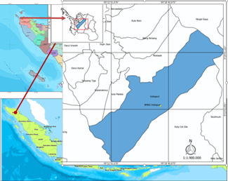
The study area for data collection carried out in this area is the Indrapuri Subdistrict, Aceh Besar District, Aceh Province, shown in Figure 1. The study was conducted for six months, starting from May to September 2019. This research monitors/surveyed rainfall data at the study location and the next step is to analyze using the SARIMA method.
2.2 Data type and source
The data used in this study is quantitative, namely monthly rainfall data between Januarys to December during the period 2003-2018. Rainfall data during this period were collected from BMKG of Indrapuri Station, Aceh Besar Regency, and Aceh Province.
2.3 Methodology
The use of the SARIMA method for the analysis of rainfall data has been described in several studies as reported by studies [28-30]. Where the equation used can be used as a guide to predict rainfall data. Analysis of rainfall data using the SARIMA method as in Eqns. (1) to (5).
ϕP (BS) ϕp(B) (1-BS)D (1-B)d Xt = ӨQ(BS) Өq(B) ɑt (1)
ϕP (BS) = 1- ϕ1BS – ϕ2B2S- ...- ϕpBPS (2)
ϕp(B) = 1- ϕ1B – ϕ2B2- ...- ϕpBp (3)
ӨQ(BS) = 1+ Ө1BS + Ө2BS+ ...+ ӨQBQS (4)
Өq(B)= 1+ Ө1B + Ө2B+ ...+ ӨqBq (5)
where, Xt is T-time series data, ϕp (B) is Eq. AR(p), Өq (B) is Eq. MA (q), ϕP (BS) is parameter of Seasonal Eq. AR(P), ӨQ (BS) is Seasonal Eq. (Q), (1-B)d is Non-seasonal differentiator, (1-BS)D is Seasonal differentiator with periods and S; ɑt is Error value.
2.4 Data stationary testing
Data is said to be stationary when the time series diagram fluctuates around a line parallel to the time axis. If the data is not stationary, the differencing process can be performed. The analysis process for differencing can be done using Eq. (6).
ΔYt = Yt – Yt – 1 (6)
where, ΔYt is Proses differencing, Yt: Observation data to and yt-1 is Observation-t on time lag 1.
Figure 1. Map of research location
2.5 Model identification
Model identification is done to get the appropriate model to predict rainfall data. The identification process can be done in two ways namely; first observation by making ACF and PACF plots. While the second way can be done by trial error. The process for general identification of ACF (Auto Correlation Function) and PACF (Partial Auto Correlation Function) as shown in Eqns. (7) and (8).
$r_k=\frac{\sum_{t=k+1}^n \, \, \, \, \left(y_t-\hat{\mathrm{y}}\right)\left(y_{t-k}-\hat{\mathrm{y}}\right)}{\sum_{t=1}^n \, \, \left(y_t-\hat{y}\right)^2}$ (7)
where, rk is Autocorrelation Coefficient, yt is Observation-t data, ŷ is Average observational data and yt-k is Observation-t on time lag k.
$\rho_k=\frac{\sum_{k=1}^n \, \, \left[\left(y_t-\hat{\mathrm{y}}\right)\left(y_{t+k}-\hat{\mathrm{y}}\right)\right]}{\sqrt{\sum\left(y_t-\hat{\mathrm{y}}\right)^2 \sum\left(y_{t+k}-\hat{\mathrm{y}}\right)^2}}$ (8)
where, ρk is Partial Autocorrelation Coefficient, yt is Observation-t data, ŷ is Average observational data and yt-k is Observation-t on time lag k.
2.6 Estimation of model parameter
The identification process can be carried out using an estimation model with parameters so that significant results can be obtained. To produce significant data, the trials conducted can use the following hypothesis.
H0: Parameter estimation=0
H1: Parameter estimation≠0
The calculated thitung is used to test whether the variable has a significant effect on the dependent variable or not. A variable will have a significant influence if the calculated thitung of the variable is greater than the ttable. Meanwhile, the calculation can be done using Eq. (9).
Test statistics:
$t_{\text {hitung }}=\frac{\phi}{\operatorname{se}(\phi)}$ (9)
Test Criteria: Reject H0 if:
$\left|t_{\text {hitung }}\right|>t \frac{\alpha}{2} n-1$ or P-value $>\alpha$ (10)
where, Φ is Parameter estimation and Se (ϕ) is Standard error parameter
2.7 Diagnostic check
At this stage, a diagnostic check is performed for the white noise test. White noise testing can be done using statistical tests from Eq. (8) with a statistical hypothesis:
H0: ρi=0, residual white noise
H1: minimal have one ρi≠0, no residual white noise
Testing at a significance level ɑ=5% can use Eq. (11).
$\mathrm{Q}=\mathrm{n}^{\prime}\left(\mathrm{n}^{\prime}+2\right) \sum_{k=1}^m \frac{r_k^2}{n^{\prime}-k}$ (11)
where, nʹ is the amount of residual, m is maximum lag time (number of parameters), rk is autocorrelation for team lag 1,2,3 ..., k and k is Lag to-k.
While for testing criteria, where accept H0 if P-value ≥ 0.05 and rejected if H0 in other conditions.
2.8 Selection of the best model
The selection of the best model is based on the size of the best model. The best model was chosen results from the smallest value of MSE (Mean Square Error). Thus, to find the value of MSE can use Eq. (12).
$\mathrm{MSE}=\frac{1}{n} \sum_{i=1}^n\left(Y_{t-} \hat{Y}_t\right)$ (12)
where, n is the amount of data, Yt is observation data at time t and Ŷt is data prediction at time t.
2.9 Prediction and comparison of prediction results with actual data
The actual data prediction can be done using the best model produced in the previous stage. Furthermore, the forecast results obtained are compared with the actual data. Then the best prediction results are chosen by category by evaluating a better model. The interpretation values Eqns. (13)-(15) for Nash-Sutcliffe Efficiency (NSE), RMSE-Observation Standard Deviation Ratio (OSDR) or RSR and PBIAS [31] are shown in Table 1.
$N S E=1-\sqrt{\frac{\sum_{i=1}^N \, \left(P o_i-P s_i\right)^2}{\sum_{i=1}^N \, \left(P o_i-\bar{P} s_i\right)^2}}$ (13)
$R S R=\sqrt{\frac{\sum_{i=1}^N \, \left(P o_i-P s_i\right)^2}{\sum_{i=1}^N \, \left(P o_i-\bar{P} s_i\right)^2}}$ (14)
$P B I A S=\frac{\sum_{i=1}^N \, \, \left(P o_i-P s_i\right) * 100}{\sum_{i=1}^N \, \, \left(P o_i\right)}$ (15)
where, Poi is data of rainfall observation, Psi is data of rainfall prediction, $\bar{P} s_i$ is mean of data rainfall prediction and N is the amount of data.
Table 1. Value interpretation of NSE, RSR and percent bias (PBIAS) [31]
|
Performance ratings |
NSE |
RSR |
PBIAS |
|
Very Good |
0.75 < NSE ≤ 1.00 |
0.00 ≤ RSR ≤ 0.50 |
PBIAS ≤ ± 25 |
|
Good |
0.65 < NSE ≤ 0.75 |
0.50 < RSR ≤ 0.60 |
± 25 ≤ PBIAS < ± 40 |
|
Satisfying |
0.50 < NSE ≤ 0.65 |
0.60 < RSR ≤ 0.70 |
± 40 ≤ PBIAS < ± 70 |
|
Not satisfactory |
NSE ≤ 0.50 |
RSR > 0.70 |
PBIAS ≥ ± 70 |
Rainfall data analysis is done directly at the location to obtain more accurate results that have been completed. These results are used to reschedule the agricultural planting period in the Greater Aceh Regency. Thus, the drought that often occurs so far after the completion of the planting period can be reduced. The results of the analysis carried out with several models that have been carried out as described as follows.
3.1 Data stationary testing
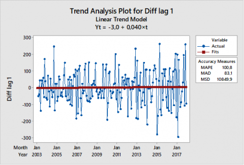
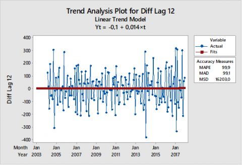
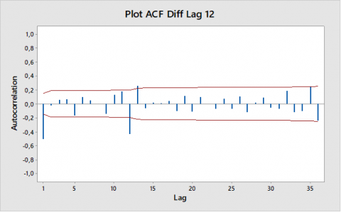
The best statistical data can be said if the lines shown are parallel to time with no repetition pattern. Analysis of trend data for the Autocorrelation Function (ACF) conducted in this study using annual rainfall data during the 2003-2017 period is shown in Figure 2. Time series (TS) data in the last five years have not shown stationary, so it must be done differencing by distinguishing non-seasonal and seasonal. So that the data that has been done differencing ACF data is seasonal and non-seasonal as shown in Figures 2 and 3. Results of the analysis of seasonal and non-seasonal rainfall data for ACF after differencing data showed a cut-off pattern. The results of rainfall data over the past five years have shown better results than in the last fifteen (15) and ten (10) years. Figure 2 (a) shows the results of non-seasonal rainfall data taken in Lag 1. While for Figure 2 (b) is the result of the analysis of non-seasonal rainfall data at Lag 12. The results of the analysis using the method described in the previous chapter show that the higher the lag tested shows better. Whereas shown in Lag 12 for the MAPE value of 99.9 lower than MAPE (Mean Absolute Percentage Error) 1 of 100.8. However, the MAD and MSD values in Lag 1 are lower than Lag 12 with values of 83.1 and 10849.9 instead of 99.1 and 16203.0.
Furthermore, data analysis was performed for seasonal rainfall data by testing 35 Lags. Tests for seasonal rainfall data are carried out to investigate the results of ACF as shown in Figure 2 (c) and (d). The results of rainfall data testing for Trend Analysis Plot (TAP) using data for the past five years show parallel time growth. However, trends for seasonal ACF show results with time series (TS). So the ACF trend needs to be done differencing, but only for seasonal lag. Its are the results of the analysis for seasonal and non-seasonal rainfall data.
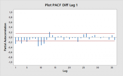
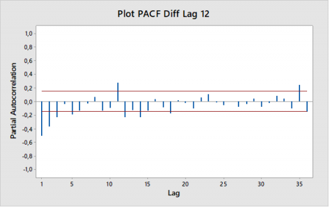
3.2 Identification mode
Identification of annual rainfall levels can be done with two PACF models as shown in Figure 3. The results of this analysis are displayed for Lag 1 and Lag 12, because both of these Lags the data displayed is easier to analysis, while the other Lags show a trend. There are the results of rainfall data after differencing. Data analysis conducted in this stage is rainfall data during the 2003-2017 period. Where the results for order 1 testing with seasonal and non-seasonal rainfall data with the model carried out at the time of differencing were respectively (0.1.1)12. In more detail, the overall results tested are shown in Table 2. Analysis results for rainfall data for the past five years have shown comparable results between lines parallel to time.
3.3 Model parameter estimation and diagnostic checks
The results of the analysis using several models show significant results for each time series with the values determined Ljung-Box shown in Table 2. The autocorrelation analysis helps detect patterns and check for randomness. Its mean lag in ACF (Autocorrelation Function) and PACF (Partial Autocorrelation Function) plot. ACF plot: it is merely a bar chart of the coefficients of correlation between a time series and lags of itself. The PACF plot is a plot of the partial correlation coefficients between the series and lags of itself. 12 shows the lags in ACF and PACF Plot. So the results of testing by applying the model as described in the previous chapter that the results of the analysis in this paper have met the requirements as stated predetermined.
Tests conducted in this study were made with three tests. Where the first test is done with rainfall data for the 2003-2017 period, the second test uses the 2008-2017 rainfall data and the third uses the 2013-2017 rainfall data. Based on the results shown in Table 2, rainfall data for the past five years has shown a cut-off or has been predicted after differencing.
3.3.1 Selection of the best model
After differencing is done by using several models, then the best selection is made based on the smallest MSE value of each model in each time series. So that the MSE results for each model selected based on the time series as shown in Table 3. The results shown in Table 3 are the smallest MSE results at the time of TS testing in each test carried out three times. The selection of MSE for testing rainfall data over the past five years 2013-2017 uses more than eight models that produce the smallest MSE value. While for the 2003-2017 data produced six models with the smallest MSE and for rainfall 2008-2017 produced five models with the smallest MSE. Thus, the 2013-2017 rainfall data shows a cut off compared to 2008-2017 and 2003-2017.
(a) Analysis of rainfall trends 2003-2017 for lag 1
(b) Analysis of rainfall trends 2003-2017 for lag 12
(c) Autocorrelation Function (ACF) plot after differencing lag 1
(d) Autocorrelation Function (ACF) plot after differencing lag 12
Figure 2. Analysis of rainfall trends
(a) Plot PACF after differencing Lag 1
(b) Plot PACF after differencing Lag 12
Figure 3. Plot PACF
Based on the results shown in Table 3, the smallest MSE value was recorded in the 2003-2017 Time series with a model using (0.0.0) (0.1.1)12 of 4343.86. For the smallest MSE results in the 2008-2017 Time series using the model (0,0,0) (0,1,2)12 amounted to 4603.71. While the smallest MSE value for the 2013-2017 Time series was arranged on the use of the model (0.0.0) (0.1.2)12 at 4628.16. Thus, these models will be used as models when testing for the next Time series prediction.
3.3.2 Prediction result
Based on the results shown in Table 3, the smallest MSE value was recorded in the 2003-2017 Time series with a model using (0.0.0) (0.1.1)12 of 4343.86. For the smallest MSE results in the 2008-2017 Time series using the model (0,0,0) (0,1,2)12 amounted to 4603.71. While the smallest MSE value for the 2013-2017 Time series was arranged on the use of the model (0.0.0) (0.1.2)12 at 4628.16. Thus, these models will be used as models when testing for the next Time series prediction. Predicted results by using the best model selection before each TSP. The results of the prediction analysis of the best models in each Time series are shown in Table 4.
This analysis was carried out using annual data between January and December. This data analysis aims to find out the actual rainfall data, TSP 2003-2017, 2008-2017 and 2013-2017. The highest actual rainfall was recorded in November at 323 and the lowest was found in August at 41. The lowest TSP (Time Series Prediction) for the period 2003-2017 was recorded in July and the highest was found in November of 73.1 and 321.8, respectively. The lowest TSP 2008-2017 data was recorded in February of 123 and the highest in December of 300.7. While for the 2013-2017 TSP the highest was recorded in December and the lowest in March were 304.2 and 18.5, respectively. Similar research results for rainfall prediction with analysis using the SARIMA model have been carried out [20]. That the use of the proposed method can the last iteration, comparable to actual observations.
3.3.3 Evaluate the best results and predictions
The results shown in Table 5 are the results of rainfall predictions from all-time series tested for 15 years, 10 years and 5 years. Then the results are evaluated using the Nash-Sutcliffe Efficiency (NSE) statistical method, RMSE-Observation Standard Deviation Ratio (OSDR) and PBIAS. This test each data group using one model. Rainfall data for the last five years shows better results than rainfall data for 10 and 15 years. Increasing the value displayed on the NSE will further reduce PBIAS so that the results obtained are more accurate. Research for rainfall prediction using the SARIMA model has also been carried out in China recently [28]. The results in their study that the SARIMA model (0.0.1)(2.0.0)12 can produce minimum average square root errors and the percentage of absolute errors finally selected for simulation in the sample.
The best accuracy model shows with highest NSE, Lowest RSR, and Highest PBIAS result Where the results displayed indicate that predictions using the 2003-2017 and 2008-2017 time series produce predictive values in the "good" category for all evaluation models tested. While the prediction results when using 2013-2017 time series data the prediction results shown are better in the "very good" category for all evaluation models tested. Based on the results of predictions obtained from this study, it can be said the results of predictions by using the number of time series data more cannot guarantee to produce more accurate data. Instead of testing using time series, data can produce more accurate and more reliable prediction results. The best prediction results displayed from the study were obtained from the use of time-series data for more recent monthly rainfall, namely during the last five years period of 2013-2017. Rainfall is very appropriate for modelling and estimating the time series of monthly rainfall data. The comparative results of the actual rainfall and prediction results as shown in Figure 4.
Similar research results for predicting rainfall trends using the SARIMA model have also been reported [23] Where the results are reported that the addition of long data cannot produce a better prediction level. In their research predictions were made to optimize annual and monthly rainfall data. Research by the ARIMA method for prediction of the influence of historical data length has also been carried out by the study [21].
Table 2. The significant value of Ljung-Box in each time series
|
Time Series |
Model |
P-value |
|||
|
Lag 12 |
Lag 24 |
Lag 36 |
Lag 48 |
||
|
2003-2017 |
(0.1.1)(0.1.1)12 |
0.217 |
0.479 |
0.396 |
0.399 |
|
(0.0.0)(0.1.1)12 |
0.307 |
0.532 |
0.429 |
0.390 |
|
|
(0.0.0)(0.2.2)12 |
0.169 |
0.389 |
0.194 |
0.165 |
|
|
(0.1.1)(0.2.2)12 |
0.145 |
0.369 |
0.164 |
0.118 |
|
|
(0.0.0)(1.2.3)12 |
0.065 |
0.127 |
0.120 |
0.085 |
|
|
(0.0.0)(1.2.2)12 |
0.295 |
0.220 |
0.095 |
0.161 |
|
|
2008-2017 |
(0.1.1)(0.1.1)12 |
0.118 |
0.320 |
0.168 |
0.109 |
|
(0.0.0)(0.1.1)12 |
0.161 |
0.343 |
0.181 |
0.093 |
|
|
(0.0.0)(0.1.2)12 |
0.111 |
0.231 |
0.091 |
0.135 |
|
|
(0.1.1)(0.2.2)12 |
0.113 |
0.215 |
0.081 |
0.072 |
|
|
(0.0.0)(1.1.1)12 |
0.204 |
0.255 |
0.151 |
0.183 |
|
|
2013-2017 |
(0.1.1)(0.1.1)12 |
0.713 |
0.950 |
0.951 |
- |
|
(0.0.0)(0.1.1)12 |
0.728 |
0.945 |
0.903 |
- |
|
|
(1.1.0)(0.1.1)12 |
0.128 |
0.496 |
0.590 |
- |
|
|
(0.1.1)(1.1.0)12 |
0.527 |
0.518 |
0.926 |
- |
|
|
(0.0.0)(0.1.2)12 |
0.164 |
0.600 |
0.781 |
- |
|
|
(0.2.1)(0.2.2)12 |
0.486 |
0.406 |
- |
- |
|
|
(0.0.0)(1.1.0)12 |
0.581 |
0.434 |
0.880 |
- |
|
|
(0.0.0)(1.1.1)12 |
0.220 |
0.123 |
0.280 |
- |
|
Table 3. MSE Value of Each Model Based on Time series
|
Time Series |
Model |
MSE |
|
2003-2017 |
(0.1.1)(0.1.1)12 |
4531.98 |
|
(0.0.0)(0.1.1)12 |
4343.86 |
|
|
(0.0.0)(0.2.2)12 |
5109.30 |
|
|
(0.1.1)(0.2.2)12 |
6072.01 |
|
|
(0.0.0)(1.2.3)12 |
4973.76 |
|
|
(0.0.0)(1.2.2)12 |
4934.28 |
|
|
2008-2017 |
(0.1.1)(0.1.1)12 |
5067.50 |
|
(0.0.0)(0.1.1)12 |
4840.87 |
|
|
(0.0.0)(0.1.2)12 |
4603.71 |
|
|
(0.1.1)(0.2.2)12 |
8394.76 |
|
|
(0.0.0)(1.1.1)12 |
4605.52 |
|
|
2013-2017 |
(0.1.1)(0.1.1)12 |
6592.51 |
|
(0.0.0)(0.1.1)12 |
6584.57 |
|
|
(1.1.0)(0.1.1)12 |
9282.25 |
|
|
(0.1.1)(1.1.0)12 |
8770.77 |
|
|
(0.2.1)(0.2.2)12 |
29424.6 |
|
|
(0.0.0)(1.1.0)12 |
8725.24 |
|
|
(0.0.0)(1.1.1)12 |
5539.53 |
|
|
(0.0.0)(1.1.1)12 |
5539.53 |
Table 4. Prediction results from the selected models in each time series
|
Month |
Rainfall Actual |
Time series prediction (TSP) 2003-2017 |
Time series prediction (TSP) 2008-2017 |
Time series prediction (TSP) 2013-2017 |
|
January |
143 |
225.3 |
197.2 |
105.4 |
|
February |
49 |
127.6 |
123.0 |
72.3 |
|
March |
83 |
156.7 |
127.0 |
18.5 |
|
April |
227 |
211.4 |
211.9 |
211.1 |
|
May |
164 |
171.6 |
198.2 |
202.5 |
|
June |
49 |
86.1 |
90.7 |
56.0 |
|
July |
52 |
73.1 |
94.3 |
69.2 |
|
August |
41 |
90.0 |
94.4 |
46.7 |
|
September |
92 |
146.6 |
126.6 |
95.5 |
|
October |
196 |
180.0 |
189.3 |
213.2 |
|
November |
323 |
321.8 |
309.0 |
298.3 |
|
December |
227 |
273.4 |
300.7 |
304.2 |
Table 5. Comparison of prediction results table for each model and time series
|
Model |
Time Series |
NSE |
RSR |
PBIAS |
Information |
|
(0,0,0) (0,1,1)12 (0,0,0) (0,1,2)12 (0,0,0) (0,1,2)12 |
2003-2017 |
0.69 (good) |
0.55 (good) |
-25.4 (good) |
Good |
|
2008-2017 |
0.73 (good) |
0.52 (good) |
-25.3 (good) |
Good |
|
|
2013-2017 |
0.84 (very good) |
0.41 (very good) |
-2.8 (very good) |
Very good |
For stationary data, seasonal factors can be determined by identifying the autocorrelation coefficients at two or three time-lags that are significantly different from zero. Autocorrelation which is significantly different from zero indicates the presence of a pattern in the data. To recognize the presence of seasonal factors, must look at the high autocorrelation. Therefore, the challenge for researchers is how to find the long time-series data or the historical data length that is closest to the pattern to be predicted. So to be able to find the long time-series data or the nearest historical data length through the predicted pattern, it must make a comparison or comparison of predictions from several historical data lengths.
Figure 4. Comparison of actual rainfall and best prediction results
The results of predictions using time series data on rainfall for 15 years (2003-2017) fall into the "good" category for 10 years (2008-2017) fall into the "good" category and for 5 years (2013-2017) fall into the "Very good" category. The results of the best model evaluation (0.0.0) (0.1.2)12 for NSE were 0.84, RSR 0.41 and PBIAS -2.8. Prediction results that are closest to the actual value are obtained from the use of time series rainfall data for 5 years with a prediction model (0.0.0) (0.1.2)12 and equation (1-B12) Xt=-2.81 (1+ 1,296 B12 - 0.575 B24) ɑt. To produce more accurate rainfall predictions in the future, further research can be done with the use of more diverse time series data. The model used for rainfall data analysis uses SARIMA. This analysis is carried out to estimate yearly rainfall data that can be used for predictions for the future. This is important to do so that future agricultural planting can be more accurate and not affected by the dry season. The accuracy of the prediction of rainfall will produce a better predictive discharge to be the basis for water resource management.
[1] Ichwana, A.A., Chairani, S. (2015). Climate trends and dynamic change of land use patterns in krueng peusangan watershed. Aceh-Indonesia. International Symposium of Geoinformatics (ISYG), Brawijaya University, Malang.
[2] Angles, S., Chinnadurai, M., Sundar, A. (2011). Awareness on impact of climate change on dryland agriculture and coping mechanisms of dryland farmers. Indian Journal Agricultural Economy.
[3] Brian, H., Zelinka, S., Castello, C., Curtis, D. (2006). Spatial analysis of storms using gis. Onerain Inc 9267 Greenback Lane Orangevale. https://proceedings.esri.com/library/userconf/proc04/docs/pap1891.pdf.
[4] Smith, J.A. (1993). Precipitation in Handbook of Hydrology. New York: Mcgraw-Hill, Inc. http://dl.watereng.ir/HANDBOOK_OF_HYDROLOGY.PDF.
[5] Stedinger, J.R., Vogel, R.M., Foufoula-Georgiou, E. (1993). Frequency analysis of extreme events. https://www.researchgate.net/publication/245641847_Frequency_Analysis_of_Extreme_Events.
[6] Hyndman, R.J., Athanasopoulos, G. (2018). Forecasting: Principles and Practice, Otexts.
[7] Lewis-Beck, M.S. (2005). Election forecasting: Principles and practice. Br J Polit Int Relations, 7(2): 145-164. https://doi.org/10.1111/j.1467-856X.2005.00178.x
[8] Ramli, I., Rusdiana, S. Basri, H., Munawar, A.A., Azelia., V. (2019). Predicted rainfall and discharge using vector autoregressive models in water resources management in the high hill takengon. IOP Conference Series: Earth and Environmental Science, 273: 012009. https://doi.org/10.1088/1755-1315/273/1/012009.
[9] Brockwell, P.J., Davis, R.A. (2016). Introduction to Time Series and Forecasting, Springer.
[10] Montgomery, D.C., Jennings, C.L., Kulahci, M. (2015). Introduction to Time Series Analysis and Forecasting. John Wiley & Sons.
[11] Box, G.E.P., Jenkins, G.M., Reinsel, G.C., Ljung, G.M. (2015). Time Series Analysis: Forecasting and Control. John Wiley & Sons.
[12] Jay, H., Barry, R., Chuck, M., Amit, S. (2014). Operation Management: Sustainability and Supply Chain Management.
[13] Suhartono. S. (2011). Time series forecasting by using seasonal autoregressive integrated moving average: Subset, multiplicative or additive model. Journal of Mathematics and Statistics, 7(1): 20-27. http://dx.doi.org/10.3844/jmssp.2011.20.27.
[14] Wang, S.W., Feng, J., Liu, G. (2013). Application of seasonal time series model in the precipitation forecast. Mathematical and Computer Modelling, 58(3-4): 677-683. https://doi.org/10.1016/j.mcm.2011.10.034
[15] Box G.E.P., Jenkins G.M., Reinsel G.C. (2008). Time series analysis: Forecasting and control, 4th ed. New Jersey. John Wiley and Sons, Inc., ISBN: 978-0470272848, p. 784.
[16] Salas J.D., Delleur J.W., Yev-Jevich V., Lane W.L. (1980). Applied modelling of hydrologic time series. littleton, colorado. Water Resource Publications, p. 484.
[17] Salas, J.D., Tabios, G.Q., Bartolini, P. (1985). Approaches to multivariate modelling of water resources time series. Journal of the American Water Resources Association, 21: 683-708. https://doi.org/10.1111/j.1752-1688.1985.tb05383.x
[18] Subbaiah Naidu, K.C.H.V. (2016). Sarima modelling and forecasting of seasonal rainfall patterns in India. International Journal of Mathematics Trends and Technology, 38(1): 15-22. http://dx.doi.org/10.14445/22315373/IJMTT-V38P504
[19] Liu, H., Li, C.X., Shao, Y.Q., Zhang X., Zhai Z., Wang, X., Qi, X.Y., Wang, J.H., Hao, Y.H., Wu, Q.H., Jiao. M.L. (2020). Forecast of the trend in the incidence of acute hemorrhagic conjunctivitis in China from 2011-2019 using the seasonal autoregressive Integrated Moving Average (SARIMA) and exponential smoothing (ETS) models. Journal of Infection and Public Health, 13(2): 287-294. https://doi.org/10.1016/j.jiph.2019.12.008
[20] Dindarloo, S., Hower, J.C., Bagherieh, A., Trimble, A.S. (2016). Fundamental evaluation of petrographic effects on coal grindability by seasonal autoregressive Integrated Moving Average (SARIMA). International Journal of Mineral Processing, 154: 94-99. https://doi.org/10.1016/j.minpro.2016.07.005
[21] Ramli, I., Rusdiana, S., Yulianur, A., Achmad, A. (2019). Comparisons among rainfall prediction of monthly rainfall basis data in Aceh using an autoregressive moving average. IOP Conference Series: Earth and Environmental Science, 365: 012008. https://doi.org/10.1088/1755-1315/365/1/012008
[22] Jeong, K., Koo, C., Hong, T. (2014). An estimation model for determining the annual energy cost budget in educational facilities using SARIMA (seasonal autoregressive Integrated Moving Average) and ANN (artificial neural network). Energy, 71: 71-79. https://doi.org/10.1016/j.energy.2014.04.027
[23] Arumugam, P., Saranya, R. (2018). Outlier detection and missing value in seasonal ARIMA model using rainfall data. Materials Today: Proceedings, 5(1): 1791-1799. https://doi.org/10.1016/ j.matpr.2017.11.277
[24] Wiredu, S., Nasiru, S. Asamoah, Y.G. (2013). Proposed seasonal autoregressive Integrated Moving Average model for forecasting rainfall pattern in the Navrongo municipality of Ghana. Journal of Environment and Earth Science, 3: 80-85.
[25] Ebenezer, A.Y., Bashiru, I.I.S., Azumah, K. (2016). Sarima modelling and forecasting of monthly rainfall in the Brong Ahafo region of Ghana. World Environment, 6: 1-9. https://doi.org/10.5923/j.env.20160601.01.
[26] Papalaskaris, T., Theologos, P., Pantrakis, A. (2016). Stohastic monthly rainfall time series analysis, modeling and forecasting in Kavala city, Greece, north-eastern Mediterranean basin. Procedia Engineering, 162: 254-263. https://doi.org/10.1016/j.proeng.2016.11.054.
[27] Tariq, M.M., Abbasabd, A.I. (2016). Time series analysis of nyala rainfall using Arima method. SUST Journal of Engineering and Computer Science, 17(1): 5-11. https://www.researchgate.net/publication/320676986_Time_Series_Analysis_of_Nyala_Rainfall_Using_ARIMA_Method.
[28] Chuang, A. (2012). Time series analysis: Univariate and multivariate methods. Technometrics, 33(1): 108-109. https://doi.org/10.1080/00401706.1991.10484777
[29] William, W.S.W., Wei, S. (2006). Time Series Analysis: Univariate and Multivariate Methods, USA, Pearson Addison Wesley, Segunda Edicion. Cap, 10: 212-235.
[30] Jobson, J.D. (2012). Applied Multivariate Data Analysis: Volume II: Categorical and Multivariate Methods. Springer Science & Business Media.
[31] Moriasi, D., Arnold, J., Van Liew, M.W., Bingner, R., Harmel, R.D., Veith, T.L. (2007). Model evaluation guidelines for quantification of accuracy in watershed simulations. Transactions of the ASABE, 50(3): 885-900. http://dx.doi.org/10.13031/2013.23153