Estimation and Analysis of Building Costs Using Artificial Intelligence Support Vector Machine

It is usually hard to accurately calculate a model using cost time series data produced by linear methods. In the construction industry, the use of linear estimation techniques is not feasible [12-16]. Cost information is used in building projects in a complex and nonlinear way. Therefore, as conventional linear estimate approaches are inappropriate for these projects, it is crucial to develop cutting-edge methodologies like artificial intelligence for estimating time series data. In order to address the weaknesses of the widely-used strategies, this research reports on the cost estimate of these projects by suggesting a new, intelligent model built on two effective methodologies.

2.1 Support vector machine

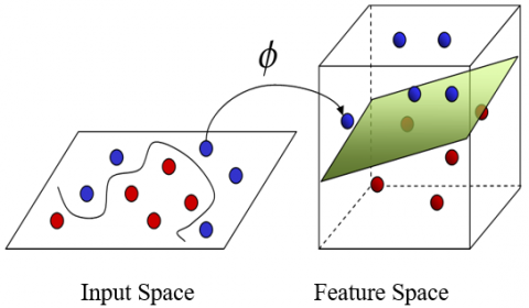
Vapnik built the first SVMs on the back of SLT in the late 1960s. However, from the middle of the 1990s, as more computer power became available, the algorithms used for SVMs began to emerge, opening the door for several real-world applications with significant outcomes [16]. As shown in Figure 1 [17], the basic SVM works with two-class issues where the data are divided by a hyperplane that is specified by a set of support vectors. For the sake of thoroughness, a basic introduction to SVM is provided below. Readers can refer to the SVM tutorials [18] for detailed descriptions. A novel training method based on the SVM called least squares support vector machines (LS-SVM) only needs the answers to a few linear equations as opposed to the regular SVM's lengthy and computationally challenging quadratic programming issue. The least squares cost function is used by the LS-SVM [19].

figure_1.png

Figure 1. Nonlinear SVM [11]

Classification: The SVM is designed to learn a unique function that categorises training instances into different groups according to the class labels that have been provided to them. This viewpoint asserts that SVMs are a category of supervised learning model that are mostly employed to address classification and regression problems [20]. By converting the input vector x into a high-dimensional feature space, SVM models developed in the new space can represent a linear or nonlinear decision boundary in the old space. A linear hyperplane can be used to partition the instances if they are linearly separable; if not, the case is nonlinearly separable [20].

Consider a given set S with n labeled training instances: $\left\{\left(\mathrm{x}_1, \mathrm{y}_1\right),\left(\mathrm{x}_2, \mathrm{y}_2\right), \ldots,\left(\mathrm{x}_{\mathrm{n}}, \mathrm{y}_{\mathrm{n}}\right)\right\}$ for the linearly separable case. Each training instance $x_j \in R^k$, for i=1, …, n, belongs to one of the two classes in comparison to its label $\mathrm{y}_{\mathrm{i}} \in\{-1,+1\}$, where $\mathrm{k}$ is the input dimension. The following equation may be used to explain the greatest margin hyperplane:

$\mathrm{y}=\mathrm{b}+\sum \mathrm{w}_{\mathrm{i}} \mathrm{y}_{\mathrm{i}} \mathrm{x}(\mathrm{i}) \mathrm{x}$     (1)

where denotes a dot product, a test example is represented by the vector x , and support vectors are represented by the vectors x(i)s. The parameters, b and $\mathcal{w}_i$ in this equation, which determines the hyperplane, must be learned by the SVM. To create a perfect hyperplane, the following sequential quadratic programming (QP) problem must be solved:

$$\text { Minimize } \frac{1}{2}\|\mathrm{w}\|^2$$  Subject to $y_i\left(w x_i+b\right) \geq 1 \quad i=1, \ldots, n$     (2)

where, the kernel function is defined as $\mathrm{K}(\mathrm{x}(\mathrm{i}), \mathrm{x})$. There are several kernels available for creating the inner products needed to construct SVMs with various nonlinear decision surfaces. The most often used kernel functions are the Gaussian radial basis function $K(x, y)=\exp \left(-1 / \delta^2(x-y)^2\right)$ and the polynomial kernel $K(x, y)=(x y+1)^d$, where, d is the degree of the polynomial kernel and $\delta^2$ is the bandwidth of the Gaussian radial basis function [20].

Regression: A version of the SVM for regression has been included in the SVMs, which have been created for general estimation and prediction applications (LS-SVM). By reducing the prediction error, LS-SVM seeks to identify a function that accurately approximates the training examples. By simultaneously attempting to maximize the flatness of the function, the danger of over-fitting is reduced when the error is minimized. One must once again resolve the following quadratic programming issue to identify an ideal hyperplane:

$$\operatorname{Minimize} \frac{1}{2}\|\mathrm{w}\|^2$$  Subject to $\left\|y_i\left(w \cdot x_i+b\right)\right\| \leq \varepsilon$     (3)

where, the value $\varepsilon \geq 0$ is the prediction error bound. If $\mathrm{f}=\langle\mathrm{w}, \mathrm{x}\rangle+\mathrm{b}$ genuinely exists and approximates all pairs $\left(x_i, y_i\right)$ with $\mathcal{\varepsilon}$ precision, then the aforementioned convex optimization problem will be achievable. The following optimization problem has restrictions that are ordinarily impossible to satisfy, thus one inserts slack variables $\varphi_{\mathrm{i}}, \varphi_{\mathrm{i}}^*$ to deal with them:

$\operatorname{Minimize} \frac{1}{2}\|\mathrm{~W}\|^2+C \sum_{\mathrm{i}=1}^l\left(\varphi_{\mathrm{i}}, \varphi_{\mathrm{i}}^*\right)$

Subject to $\left\{\begin{array}{c}y_i-\left\langle w, x_i\right\rangle-b \leq \varepsilon+\varphi_i \\ \left\langle\mathrm{w}, \mathrm{x}_{\mathrm{i}}\right\rangle+\mathrm{b}-\mathrm{y}_{\mathrm{i}} \leq \varepsilon+\varphi_{\mathrm{i}}^* \\ \varphi_{\mathrm{i}}, \varphi_{\mathrm{i}}^* \geq 0\end{array}\right.$     (4)

The trade-off between f flatness and the maximum allowed deviation, $\varepsilon$, is calculated using the constant C. This optimization problem may be built as a dual problem by building the Lagrangian function:

$$\begin{aligned}\mathrm{L} & =\frac{1}{2}\|\mathrm{w}\|^2+\mathrm{C} \sum_{\mathrm{i}=1}^{\mathrm{l}}\left(\varphi_{\mathrm{i}}, \varphi_{\mathrm{i}}^*\right)-\sum_{\mathrm{i}=1}^{\mathrm{l}} \lambda_{\mathrm{i}}\left(\varepsilon+\varphi_{\mathrm{i}}-\right. \\\mathrm{y}_{\mathrm{i}} & \left.+\left\langle\mathrm{w}, \mathrm{x}_{\mathrm{i}}\right\rangle+\mathrm{b}\right)-\sum_{\mathrm{i}=1}^{\mathrm{l}} \lambda_{\mathrm{i}}^*\left(\varepsilon+\varphi_{\mathrm{i}}^*-\mathrm{y}_{\mathrm{i}}+\left\langle\mathrm{w}, \mathrm{x}_{\mathrm{i}}\right\rangle-\right.\end{aligned}$$ b) and $\lambda_{\mathrm{i}}, \lambda_{\mathrm{i}}^* \geq 0$     (5)

Solving the Lagrangian, one provides the optimal solutions $\mathrm{w}^*$ and $\mathrm{b}^*$:

$\begin{aligned} \mathrm{b}^*=\mathrm{y}_{\mathrm{i}}-\left\langle\mathrm{w}, \mathrm{x}_{\mathrm{i}}\right\rangle-\varepsilon, & 0 \leq \lambda_{\mathrm{i}} \leq \mathrm{c}, \mathrm{i}=1, \ldots, \mathrm{l}, \\ \mathrm{~b}^*=\mathrm{y}_{\mathrm{i}}-\left\langle\mathrm{w}, \mathrm{x}_{\mathrm{i}}\right\rangle+\varepsilon, & 0 \leq \lambda_{\mathrm{i}}^* \leq \mathrm{c}, \mathrm{i}=1, \ldots, \mathrm{l}\end{aligned}$     (6)

For nonlinear issues, the inner products can be changed by appropriate kernels, much like in classification. Enforcing the upper limit C on the absolute value of the coefficients $\mathrm{w}_{\mathrm{i}} \mathrm{s}$ allows us to keep an eye on the trade-off between reducing prediction error and maximizing the flatness of the regression function. The function may match the data more closely the greater C. The approach essentially does the least absolute-error regression with the coefficient size restriction in the degenerate situation where ε=0, regardless of the amount of C. In contrast, if is big enough, the error decreases to zero, and the algorithm returns the flattest curve that contains the data, regardless of the amount of C [20-22].

2.2 Cross-validation technique

Cross-validation [23] is a well-known technique for calculating generalisation mistakes. Among various cross-validation techniques, the k-Fold cross-validation approach is taken into consideration in this study. K-Fold cross-validation is one way to enhance the holdout strategy. Each of the k subgroups of the dataset uses the holdout method. Every time, one of the k subsets is used as the test set, and the remaining k-1 subsets are used to create the training set. Next, the average error over all k trials is calculated. The main benefit of this method is that it doesn't matter how the data is split up.

Each data set appears k times in the training set and exactly once in the test set. The variability of the resulting estimate diminishes as k is increased. By randomly dividing the data into test and training sets k times, this strategy may be changed. An example of how neural network architectures may be utilised to get the best generalisation is the k-fold cross-validation approach. In the pertinent literature, 3 and ten-fold cross-validation approaches were advised to estimate practical applications [24].

2.3 Intelligent proposed model

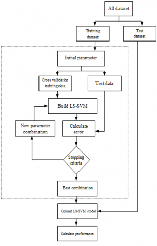
The proposed model is based on the LS-SVM and cross-validation, two effective techniques. The input-output mapping in this model is managed by the LS-SVM, which focuses on the features of cost data in building projects. The LS-SVM is trained using k-fold cross-validation to provide accurate findings and to enable a more realistic evaluation of the accuracy by splitting the whole dataset into numerous training and test sets. The suggested intelligent model may be a mix that is both suitable and efficient computationally for cost estimation of construction projects. The recommended model's steps are as follows: dividing the data into training and test sets is Stage 1: The test set is used to evaluate the model's performance after the training set has been used to create the LS-SVM model. Stage 2: Instructional data the model uses sequential data as training data. To help prevent numerical difficulties, the training data are now normalised into the same domain (0, 1) and the sequential data represents the desired attributes. The function used it to normalise data is demonstrated in the following illustration:

$x_{\text {sca }}=\frac{x_i-x_{\min }}{x_{\max }-x_{\min }}$     (7)

All the variables have no dimensions as a result of this change. Stage 3: Instruction in LS-SVM This step manages input-output mapping using the LS-SVM. The Gaussian radial basis function kernel is employed as a logical alternative [12, 20]. Using the k-fold cross-validation approach on the training data set, the LS-SVM training is done to build the prediction model.

Fitness definition: Chen and Wang [21] assert that although the training dataset's fitness may be easily calculated, it is prone to over-fitting.

This problem is solved using the k-fold cross-validation technique. This technique divides the training dataset into k subsets at random, then uses the k-1 subset as the training set to construct the regression function with the specified set of parameters $\left(\mathrm{C}_{\mathrm{i}}, \delta_{\mathrm{i}}\right)$. The final set is taken into account for validation. The preceding procedure is repeated k times. As a result, the fitness function is defined by the MAPECV of the k-fold trans procedure on the training dataset:

Fitness $=\min \mathrm{f}=\mathrm{MAPE}_{\mathrm{cv}}$    (8)

$\operatorname{MAPE}_{\mathrm{cv}}=\frac{1}{\mathrm{l}} \sum_{j=1}^1\left|\frac{y_j-\widehat{y}_j}{\mathrm{y}_{\mathrm{j}}}\right| \times 100 \%$    (9)

where, y_j is the actual value; $\widehat{y_j}$ are the validation value and l is the number of subsets. The solution with a smaller $\mathrm{MAPE}_{\mathrm{cv}}$ of the training, the dataset has a smaller fitness value. Stage 4: The LS-SVM parameters are supplied in this stage so that the estimations may be made. Choose the best parameter settings to construct the LS-SVM model in Stage 5: LS-SVM model with the test dataset substituted to achieve the estimation values. Through testing performance, it is possible to validate the LS-SVM model's estimated capacity by taking into account performance criteria to compute the error between real and estimates values. The structure of the suggested intelligent model is shown in Figure 2. To reduce the MAPECV during prediction iterations, this model is used to try to optimize the LS-parameter SVM's combinations.

figure_2.png

Figure 2. The proposed LS-SVM model

Table 2. Description of qualitative factors for conceptual cost estimating

Table 3. Overall comparative results

figure_4.png

Figure 4. Comparison of accuracy for proposed model, EFNIM, and NL cost estimation models

figure_5.png

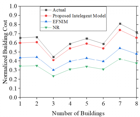
Figure 5. Examples illustrate the suggested model and two more well-known methods

MAPE and MSE often reflect accuracy as a percentage in statistics. According to this model, MAPE = 0.625 for LS-SVM, 2.214 for EFNIM, and 3.935 for NL indicating that the LS-SVM has a lower and greater percentage error than EFNIM and NR, respectively. The wide applicability of the prediction model is measured by the coefficient of determination R2, which quantifies how well data points fit a curve or a line. When represented as a percentage, R2 computes how much of the variance in the output response can be attributed to the model's predictors. R2 values fall within the range [0,1]. As shown in Figure 4, the value R2= 0.9147 for our cleverly developed model may be understood as follows: about 91% of the variation in the response is attributable to the selected predictors, and the remaining 9% is related to unknown variability.

Here, it is important to emphasize that since various types of predictive models may be appropriate depending on the type of relationship between the predictors and the dependent variable, it is best to test them all out to find the one that best fits our data and provides the most accurate predictions. The authors confirmed that the cross-validation approach was well suited for trustworthy estimation after obtaining pleasing results with LS-SVM with an error of less than 9%.

As shown in Figure 5, the prediction made using the suggested model yields results that are adequate. The minimum three indices in the final prediction results of the suggested model show strong performance and adaptability to the conceptual building cost in the construction sector. Project managers may assess construction projects appropriately, particularly in feasibility studies, by utilizing the suggested model. Additionally, it raises the likelihood that building projects will be successful.