Ranu![]() | Nitin Kumar Mishra*
| Nitin Kumar Mishra*![]()
© 2023 IIETA. This article is published by IIETA and is licensed under the CC BY 4.0 license (http://creativecommons.org/licenses/by/4.0/).
OPEN ACCESS
For carbon emission, this research study investigates a Mathematical inventory model with time, advertising, and inventory-dependent demand patterns. The main objective of this research study is to keep the total cost of retailers as well as suppliers and carbon emissions as low as possible. With collaboration and without collaboration, two cases are discussed in this proposed model. Within the first case, retailers and suppliers are not regarded as collaborators, whereas in the second case, collaboration is recognized. The optimality of the planned inventory management model is explained mathematically and theoretically in both situations. The algorithm of the mathematical solution was also properly discussed and the effects of altering various parameters are numerically studied to conduct a sensitivity analysis with the help of Mathematica software version 12. To demonstrate this model, a mathematical illustration, and a tabular and graphical representation, have been also provided. Ultimately, this model reaches a flourishing managerial suggestion and conclusion.
collaboration, advertising demand, and carbon emission
Global temperature rise is the effect of greenhouse gas emissions and even some living beings. Kaya identity also plays a suitable role in the direction of Climate change that had received a great deal of attention in past few years. A worldwide awareness about environmental conservation and protection is encouraging many more researchers, organizations, and other government agencies to create and maintain an eco-friendly as well as a negligible emission management system for supply chains. Kaya identity plays a role to calculate the impact of different factors of the supply chain on carbon emission [1]. Therefore, we rely on the kaya identity equation to calculate the amount of carbon emission.
$\mathrm{Co}_2=\left(\frac{G D P}{\text { Population }}\right)\left(\frac{E C}{G D P}\right)\left(\frac{\mathrm{Co}_2}{E C}\right) *$ Population
The entire value of all products and services generated in a country in a given year is known as the gross domestic product (GDP). GDP quantifies the monetary worth of final goods and services produced in a country over a specified duration, it may be quarterly or yearly.
Everyday activities like-Heating, cooling, electricity supply, and transportation are all dependent on efficient and reasonable energy services. All economic sectors, from business and industry to agriculture, rely on energy to function properly and effectively. Energy intensity is a ratio of the volume of energy required to produce one unit of GDP and can be used to estimate a country's energy efficiency.
The total energy consumed (EC) by end-users, such as households and businesses, industry, and modern agriculture, is referred to as final energy consumption in cooling, heating, and fossil fuel. It is the energy that achieves by the final consumer, except for energy used by the energy sector that produced emissions in large quantities. Our research work mainly focuses on carbon emission during supply chain processes such as holding (heating, refrigeration), and carbon emission due to transportation.
In inventory management, Khan et al. [2] advertising a new product or modified goods plays an extremely important role because it raises product awareness for customers to buy something, retailer, supplier, and even manufacturer, all advertise their new products, and also when a modified product from an old to new, they also advertise it. In this way, the advertisement plays an important role in increasing the demand for any product and from which we can say that the demand for any product on the day depends absolutely on its advertisement. Therefore, the advertisement will increase the product demand and the product will be sold out very soon. For retailers and suppliers to enhance customer demands is a challenging feat. That idea would be great in the case of perishable items, fashionable products and those items that are reaching their expiring date, where their life span is short. Due to carbon emissions and advertisements, demand for products will undoubtedly be influenced. Advertisement is one of the most effective promotional approaches to raise awareness about a product's popularity among all classes of consumers. There are many different ways to do advertising, in today's new technology, people advertise their new products or old to new through mass media to stimulate a larger group of customers to buy their products.
In this regard they aware customer about new products, about their price and extra information about their quality. All the players in supply chain management advertise in different ways to increase the demand for their products, for this, they advertise through different media like newspapers, posters, and television. Moreover, in the advertisement, they show the quality of the product. and at the same time, the good quality attracts the customer to buy the item very much. In the case of carbon emission, it has become very important to advertise carbon-free products, so that customers buy the carbon-free product and through which we can reduce the amount of carbon.
Therefore carbon emission with advertisement demand has become an integral part of our proposed work.
Our proposed model is a way to reduce carbon footprint and optimize the total cost of suppliers and retailers. As a result of this model, we have driven the average credit rate, the total cost of the supplier, and the total cost of the retailer are very sensitive to the deterioration rate. Another important outcome is that the average credit rate, the total cost of the supplier, and the total cost of the retailer are highly sensitive to the advertisement-dependent demand.
The vast majority of the rest of this manuscript is structured as follows. A review of the existing literature has been carried out in Section 1. The Assumptions and notations of this manuscript are presented in Section 2, and the Mathematical study and their calculating work are provided in Section 3. The sensitivity study in the graphical and tabular form is described in Section 4. Section 5, contains the managerial findings and conclusion of SCM in the context of carbon taxes.
Kaya's identity, initially expressed by Kaya [1] and eventually formally accepted by some others is the combination of four factors: emissions per unit of energy expenditure; population; per capita income and energy intensity per unit of Manufacturing output Kaya, 1989 also can be presented as follow.
$\mathrm{Co}_2=\left(\frac{G D P}{\text { Ppopulation }}\right)\left(\frac{E C}{G D P}\right)\left(\frac{\mathrm{Co}_2}{E C}\right) *Population$
Since supply chain processes account for the majority of carbon emissions, so many governments have enacted carbon taxes to encourage energy efficiency and emission reduction. In this context, the effects of carbon taxes on supply chains become topics of discussion. Zhou et al. [3] traditionally supply chains have concentrated exclusively on economic gain only. but modern technology is focusing on sustainability. Supply chains are greatly influenced by carbon taxes. Because of this need to take into account the local, national, and worldwide ecosystems as well as the widening environmentalism of the general populace. According to Liu et al. [4], producers were compelled to select low-emitting techniques after the carbon tax was elevated to a certain level. Carbon taxes may also be advantageous for manufacturers, suppliers and retailers as well as for improved environmental processes. Benjaafar et al. [5] studied that a carbon tax implemented as part of a supply chain was able to accomplish the two main goals of lowering costs and emissions. Because of this, studies have discovered that an appropriate carbon tax technique can help to achieve supply chain social, economic, and ecologic collaboration. In a two-level supply chain with a carbon tax, Cheng et al. [6] presented a collaborative model approach in which the retailer and manufacturer freely decided on collaborative carbon reduction activities. On the whole, it was determined that the carbon tax encouraged supply chain participants' joint efforts and enhanced the environment and economic performance. Park et al. [7] explained that a carbon tax was more impactful in balancing the exchange between public welfare, environmental conservation, and economic growth. From the above literature to study of carbon tax become an integral part of our proposed model.
Khan et al. [2] investigated that the advertisement of an item is directly associated with the demand. For this purpose, Goyal and Gunasekaran [8], Bhunia and Maiti [9], Shah and Pandey [10], Bhunia and Shaikh [11], Shah et al. [12], Bhunia and Shaikh [13], Shaikh et al. [14], Mishra [15], Khan et al. [2], Panda et al. [16], and many others established inventory models that took into account the effect of advertising on sales. So the retailer, supplier, and manufacturer must determine the advertisement process before the sales period. Understanding from this review of research articles, it is found that no researcher has considered an advertisement, time, and inventory-dependent demand in the finite period horizon which is unique in itself.
The supply chain covers the entire process of producing and selling essential goods. Manufacturers, suppliers, transports, warehouses, retailers, and customers are all part of the supply chain. A process by which natural resources or raw materials are turned into finished items and then sold to end-users or customers. Moreover, the majority of the available conventional literature did not analyze credit terms coordination and collaboration. However, supply chain participants such as suppliers, retailers, and manufacturers are all affected by one another. A collaborative approach to supply chain management is necessary for beneficial and effective supply chain management. So, in past few years, few such as Wu and Zhao [17], Singh et al. [18], Kim and Sarkar [19], and Barman et al. [20] researchers have begun concentrating their attention on supply chain collaboration with credit terms as a beneficial framework for retailers and supplier. In today's global world, an institution's or business owner's primary aim is to optimize overall value simultaneously and also emphasize carbon emission reduction that can be achieved by coordinating different strategies among supply chain participants. To extend the entire supply chain, a lot of work has been conducted. Multiple parameters are used to enhance supply chain efficiency. Therefore, the most pressing issues today are supply chain management for coordination as well as without coordination and carbon emission for Advertisement, time, and inventory demand underneath finite planning.
According to Daryanto et al. [21], transportation-related carbon output is determined by the amount of fuel used by the vehicle, the amount of fuel discharged, and the distance travelled. Also, discuss that fuel consumption energy is affected by transportation and emission strategy side by side total cost and amount of emission are also affected. In inventory control reducing global warming and carbon emission only through green farming is a very difficult task. For that, we have to take the help of advertisement technology and carbon regulations. advertisement technology and carbon regulations can help us to reduce total costs, carbon emissions, and global warming. We have learned from here that reducing carbon emissions and the total cost will have a positive impact on global warming as well as profit. facing these challenges, there has been very little study before this that has described carbon emission in the supply chain for advertisement, time and carbon-dependent demand underneath finite planning horizon. Hence this research provides a joint decision on inventory control with carbon emission. Various parameters such as Advertisement, time and inventory-dependent demand, and carbon emission due to refrigeration and transportation technology are considered to design a long-term supply chain.
Table 1. Comparison of literature
|
Article |
Inventory dependent demand |
Advertisement dependent demand |
Collaboration |
Carbon Emissions cost |
Transportation cost |
Finite planning horizon |
|
Benjaafar et al. [5] |
× |
× |
√ |
√ |
× |
× |
|
Cheng et al. [6] |
× |
× |
× |
√ |
× |
× |
|
Khan et al. [2] |
× |
√ |
× |
√ |
× |
× |
|
Mishra [15] |
× |
√ |
× |
√ |
√ |
× |
|
Park et al. [7] |
× |
× |
× |
√ |
× |
× |
|
Wu and Zhao [17] |
√ |
× |
√ |
× |
× |
√ |
|
Singh et al. [18] |
√ |
× |
√ |
× |
× |
√ |
|
Daryanto et al. [21] |
× |
× |
× |
√ |
√ |
× |
|
This Paper |
√ |
√ |
√ |
√ |
√ |
√ |
Research problem:
This article considers linear time-dependent, inventory-dependent, and advertisement-dependent demand with carbon emission regulation. The main objective is to properly analyze the economic as well as market scenario for some specific goods that are newly launched products, clothes, permissible items, fashionable items, and fast-moving consumer goods near deterioration or expiration date. Their demand rises or diminished according to time, inventory and advertisement. The trade-credit period offered by the supplier to its retailers for his purchases is considered under the Finite planning horizon (FPH). The collaboration of suppliers and retailers with carbon regulation is being considered. Based on the above literature, we have an idea that this will be a novel work under a finite planning horizon. Nobody has taken this problem in a finite planning horizon.
Notations:
The following are now the relevant factors only for the retailer and supplier:
Or – Total cost for placing an order (\$/order)
a - Initial demand for marketing (per yr.)
b - Demand that depends upon a time (per yr.)
hc – Cost for managing inventory in the warehouse (\$/un.)
$\Theta$ – Demand that is dependent upon inventory
Wp – Total wholesale price of items (\$/unit)
Qi – Total amount of shipments per replenishment process (units)
$T_{I N D}^r$ – The total cost of the retailer when no coordination occurs (\$/time unit)
$T_{J T}^r$ – The total cost of the retailer when coordination occurs (\$/time unit)
$T_{I N D}^S$ – The total cost of the retailer when no coordination occurs (\$/time unit)
$T_{J T}^S$ – The total cost of the retailer when coordination occurs (\$/time unit)
The following are now the relevant factors only for carbon emission:
$\hat{c}$ - Fixed amount of carbon emission
$\hat{h}_c$ - Amount of carbon emission associated with the refrigerator consumed energy during the holding
$\hat{P}_r$ - Varying carbon emissions due to the managing of each unit
ρ - Demand depend upon the amount of carbon emission
CO2 - Amount of carbon emission
τ - Carbon emission price conducted by the government
Sc- Total setup cost of supplier
Cp- its purchase price per unit ($/unit)
h - It denotes the capital cost ($/unit/yr.)
δ - the rate of the credit period.
Now, the following are the decision variables:
n - No replenishment cycles
T - Time planning horizon (Yr.)
Ti - Length of each cycle during placing an order (time/ unit)
ti - A timeframe for placing an order (time unit)
A - Advertising and marketing frequency
$\alpha$ - marketing and advertising demand function fluctuation
Transportation variables:
vc - The variable cost of fuel consumed by the retailer during transportation depends upon the fuel consumption (\$/litre)
e2 - Retailer’s additional (refrigeration) carbon emission cost from transporting one unit item (\$/unit/km)
e1 - Charge of carbon dioxide emissions from retail transportation (\$/km)
C1 - Fuel usage of a retailer's vehicle when it has been empty (litres per kilometre)
C2 - Retailer's additional (refrigeration and vehicle services) transportation energy consumption for every per ton of payload (litre/km/ton)
d - Distance covered from supplier to retailer (km)
Fc - Transportation fixed cost when order is placed by the retailer (\$)
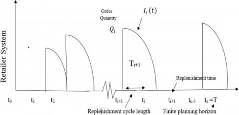
In this Phase, a mathematical explanation with no shortages of this manuscript for a finite planning period is formulated. Using the assumptions and notations mentioned in the previous phase, the following basic inventory details over the finite planning horizon. Demand is considered advertisement, inventory, carbon and time-dependent. The inventory declines eventually, usually to meet the demand and with advertising of the product. The shift in inventory level over time ($t$) during the time interval $\boldsymbol{t}_{\boldsymbol{i}} \leq \boldsymbol{t} \leq \boldsymbol{t}_{i+1}$ is defined by the differential Eq. (1).
$\frac{\mathrm{dI}_i(t)}{\mathrm{dt}}=-A^\alpha\left(a+\mathrm{bt}-\rho C o_2\right)-\theta \mathrm{I}_i(t)$ (1)
where, ti≤t≤ti+1.
Figure 1. Graphical representation of inventory level
Now, Eqns. (2)-(5) represent the demand rate, inventory level, order quantity and holding cost given below. Labelled Figure 1 depicts the rise and fall of inventory.
$\mathrm{D}\left(\mathrm{t}, \theta, \mathrm{A}, C o_2\right)=A^\alpha\left(a+\mathrm{bt}-\rho C o_2\right)+\theta \mathrm{I}_i(t)$ (2)
where, c > 0, d ≥ 0, and t is positive.
When Ii(ti+1)=0 and Ii(ti)=Qi.
$I_i(t)=\int_t^{t_{i+1}} A^\alpha\left(a+\mathrm{b} * \mathrm{u}-\rho C o_2\right) e^{\theta(u-t)} \mathrm{du}$ (3)
The order quantity for ith cycles:
$Q_i=I_i\left(t_i\right)=\int_{t_i}^{t_{i+1}} A^\alpha\left(a+\mathrm{bt}-\rho C o_2\right) e^{\theta\left(\mathrm{t}-\mathrm{t}_i\right)} \mathrm{d} t$
Ordering cost:
$O_c=\mathrm{n} * O_r$ (4)
Holding cost:
$H_c$$=\sum_{i=0}^{n-1} h_c \int_{t_i}^{t_{i+1}} \int_t^{t_{i+1}} A^\alpha\left(a+\mathrm{bt}-\rho C o_2\right) e^{\theta(u-t)} d u d t$ (5)
Carbon emission cost doesn't include carbon emission due to transportation. According to Benjaafar et al. [5], Xiang and Lawley [22], and Shi et al. [23] and Mishra and Ranu [24], $\hat{c}$ is fixed carbon emissions involved with putting an order (carbon emissions caused by transportation), $\hat{P}_r$ varying carbon emissions due to the management of each unit, and $\widehat{h_c}$ is carbon emissions associated with refrigerator-consumed energy in the storage of each unit. As a result, the total amount of carbon emissions for each replenishment process is represented by Eq. (6) given below.
$C E=\hat{c}+\sum_{i=0}^{n-1} \hat{P}_r * Q_i+\widehat{h_c} \int_{t_i}^{t_{i+1}} \int_t^{t_{i+1}} A^\alpha(a+$$\left.\mathrm{bt}-\rho C o_2\right) e^{\theta(u-t)} d u d t$ (6)
The Retailer’s transportation cost considers the fixed and variable transportation costs and carbon emissions due to FEC during refrigeration. Therefore Eq. (7) represents the transportation cost given below.
$\begin{gathered}T c=F_c+2 \mathrm{~d} v_c C_1+\mathrm{d}^* v_c C_2 \int_{t_i}^{t_{i+1}} A^a\left(a+\mathrm{bt}-\rho C o_2\right) e^{\theta\left(\mathrm{t}-\mathrm{t}_i\right)} \mathrm{d} t+2 \mathrm{~d} e_1+\mathrm{d} \\ e_2 \int_{t_i}^{t_{i+1}} A^a\left(a+\mathrm{bt}-\rho C o_2\right) e^{\theta\left(\mathrm{t}-\mathrm{t}_i\right)} \mathrm{d} t\end{gathered}$ (7)
The total individual cost of the retailer, supplier and order quantity in the case of no collaboration is given by the Eqns. (8), (9) and (10).
$\begin{gathered}T_{I N D}^r=n_1 * O_r+\hat{c}+\left\{\frac{\left(h_c+\tau \hat{h}_c\right)}{\theta}+W_p+\hat{P}_r+\mathrm{d} * v_c C_2+\mathrm{d} e_2\right\} \sum_{i=0}^{n_1-1} \int_{t_i}^{t_{i+1}} A^\alpha(a+\mathrm{bt}- \\ \left.\rho C o_2\right) e^{\theta\left(\mathrm{t}-\mathrm{t}_i\right)} \mathrm{d} t-\frac{A^\alpha\left(h_c+\tau \hat{h}_c\right)}{\theta}\left(a T+\frac{1}{2} b T^2\right)+F_c+2 \mathrm{~d} v_c C_1+2 \mathrm{~d} e_1\end{gathered}$ (8)
$T_{I N D}^S=n_1^* * S_c+C_p * \sum_{i=0}^{n_1^*-1} \int_{t_i}^{t_{i+1}} A^\alpha\left(a+\mathrm{bt}-\rho C o_2\right) e^{\theta\left(\mathrm{t}-\mathrm{t}_i\right)} \mathrm{d} t$ (9)
$Q_{\text {IND }}=\sum_{i=0}^{n_1^*-1} Q_i^*$ (10)
Now, the joint total cost of the retailer, supplier and order quantity in the case of collaboration is given by (11), (12) and (13).
$\begin{gathered}T_{J T}^s=n_2 *\left(S_c+O_r\right)+C_p * \sum_{j=0}^{n_2-1} \int_{t_i}^{t_{i+1}} A^\alpha\left(a+\mathrm{b} \mathrm{t}-\rho C O_2\right) e^{\theta\left(\mathrm{t}-\mathrm{t}_i\right)} \mathrm{d} t+\left\{\frac{\left(h_c+\tau \hat{h}_c\right)}{\theta}+W_p+\hat{P}_r+\mathrm{d} * v_c C_2+\mathrm{d} e_2\right\} \\ \sum_{i=0}^{n_2-1} \int_{t_i}^{t_{i+1}} A^\alpha\left(a+\mathrm{bt}-\rho C o_2\right) e^{\theta\left(t-t_i\right)} \mathrm{d} t-\frac{A^\alpha\left(h_c+\tau \hat{h}_c\right)}{\theta}\left(a T+\frac{1}{2} b T^2\right)+F_c+2 \mathrm{~d} v_c C_1+2 \mathrm{~d} e_1- \\ T_{I N D}^r\left(n_1^*, t_0, t_1^*, \ldots \ldots \ldots t_{n_1}^*\right)\end{gathered}$ (11)
$Q_{J T}=\sum_{j=0}^{n_2^*-1} Q_j^{\prime *}$ (12)
$\begin{gathered}T_{J T}^r=n_2 * O_r+\hat{c}+\left\{\frac{\left(h_c+\tau \hat{h}_c\right)}{\theta}+W_p+\hat{P}_r+\mathrm{d} * v_c C_2+\mathrm{d} e_2\right\} \sum_{i=0}^{n_1-1} \int_{t_j}^{j_{j+1}} A^\alpha(a+\mathrm{bt}- \\ \left.\rho C o_2\right) e^{\theta\left(\mathrm{t}-\mathrm{t}_j\right)} \mathrm{d} t-\frac{A^\alpha\left(h_c+\tau \hat{h}_c\right)}{\theta}\left(a T+\frac{1}{2} b T^2\right)+F_c+2 \mathrm{~d} v_c C_1+2 \mathrm{~d} e_1- \\ T_{I N D}^r\left(n_1^*, t_0, t_1^*, \ldots \ldots \ldots t_{n_1}^*\right)\end{gathered}$ (13)
The credit period offered by the supplier to the retailer is given by Eqns. (14)-(16):
$\delta=T_{J T}^r\left(n_2^{\prime *}, t_0, t_1^{\prime *}, \ldots \ldots \ldots . t_{n_2}^{\prime *}\right)-T_{I N D}^r\left(n_1^*, t_0, t_1^*, \ldots . \ldots . . t_{n_1}^*\right) / \sum_{j=0}^{n_2^*-1} h\left(t_{\mathrm{j}+1}^{\prime *}-t_{\mathrm{j}}^{\prime *}\right) Q_j^{\prime *}$ (14)
$\begin{gathered}\delta_{\max }=T_{I N D}^s\left(n_1^*, t_0, t_1^*, \ldots \ldots \ldots . t_{n_1}^*\right)-n_1^* * S_c-C_p * \sum_{i=0}^{n_1^*-1} \int_{t_i}^{t_{i+1}} A^a(a+ \\ \left.\mathrm{bt}-\rho C o_2\right) e^{\theta\left(\mathrm{t}-\mathrm{t}_i\right)} \mathrm{d} t / \sum_{j=0}^{n_2^*-1} h\left(t_{\mathrm{j}+1}^{\prime *}-t_{\mathrm{j}}^{\prime *}\right) Q_j^{\prime *}\end{gathered}$ (15)
$\delta_{\min }=T_{J T}^r\left(n_2^{\prime *}, t_0, t_1^{\prime *}, \ldots \ldots \ldots . t_{n_2}^{\prime *}\right)-T_{I N D}^r\left(n_1^*, t_0, t_1^*, \ldots \ldots \ldots . t_{n_1}^*\right) / \sum_{j=0}^{n_2^*-1} h\left(t_{\mathrm{j}+1}^{\prime *}-t_{\mathrm{j}}^{\prime *}\right) Q_j^{\prime *}$ (16)
The average of the credit period which is beneficial for both retailer as well as the supplier has given by Eq. (17).
where we know that $\bar{\delta}=\frac{\delta_{\min } \, \,+\delta_{\max }}{2}$ (17)
Final total cost after introducing the average credit period for both retailer as well as supplier and order quantity is given by Eqns. (18)-(19).
$\bar{T}_{J T}^r=T_{J T}^r\left(n_2^{\prime *}, t_0, t_1^{\prime *}, \ldots \ldots \ldots . t_{n_2}^{\prime *}\right)-\sum_{j=0}^{n_2^*-1} \bar{\delta} h\left(t_{\mathrm{j}+1}^{\prime *}-t_{\mathrm{j}}^{\prime *}\right) Q_j^{\prime *}$ (18)
$\bar{T}_{J T}^s=n_1^* * S_c+\sum_{i=0}^{n_1^*-1} C_p Q_i^*+\sum_{i=0}^{n_2^*-1} \bar{\delta} h\left(t_{\mathrm{j}+1}^{\prime *}-t_{\mathrm{j}}^{\prime *}\right) Q_j^{\prime *}$ (19)
The value of Hessian matrix as discussed in researches [19] and [25] has to be shown as positive definite after solving, for $T_{I N D}^r$ to be minimum.
Now, replenishment time intervals are obtained with the help of Eq. (20) which is the derivative of Eq. (8).
$\begin{gathered}\frac{\partial T_{I N D}^r}{\partial t_i}=A^\alpha\left(a+\mathrm{b} t_i+\rho C o_2\right)\left(e^{\theta\left(\mathrm{t}_i-t_{i-1}\right)}-1\right)- \\ \theta \int_{t_i}^{t_{i+1}} A^\alpha\left(a+\mathrm{bt}-\rho C o_2\right) e^{\theta\left(\mathrm{t}-\mathrm{t}_i\right)} \mathrm{d} t\end{gathered}$ (20)
where, i=1,2,3…………n.
Theorem. If $t_i$ satisfy inequations (i) $\frac{\partial^2 T_{I N D}^r}{\partial t_i^2} \geq 0$ (ii) $\frac{\partial^2 T_{I N D}^r}{\partial t_i^2} \geq\left|\frac{\partial^2 T_{I N D}^r}{\partial t_i t_{i-1}}\right|+\left|\frac{\partial^2 T_{I N D}^r}{\partial t_i t_{i+1}}\right|$ for all i= 1,2 , 3 ………. $\mathrm{n}_1$ then $\nabla^2 T_{I N D}^r$ is positive definite.
$\begin{gathered}\frac{\partial^2 T_{I N D}^r}{\partial t_i^2}=\theta A^\alpha\left(a+\mathrm{b} t_i-\rho C o_2\right) e^{\theta T_i}+\theta A^\alpha(a+ \\ \left.\mathrm{b} t_{i+1}+\rho C o_2\right) e^{\theta T_{i+1}}+A^\alpha b\left(e^{\theta T_i}-e^{\theta T_{i+1}}\right)\end{gathered}$ (21)
$\frac{\partial^2 T_{I N D}^r}{\partial t_i \partial t_{i-1}}=-\theta A^\alpha\left(a+\mathrm{b} t_i-\rho C o_2\right) e^{\theta T_i}$ (22)
Similarly,
$\frac{\partial^2 T_{I N D}^r}{\partial t_i \partial t_{i+1}}=-\theta A^\alpha\left(a+\mathrm{b} t_i-\rho C o_2\right) e^{\theta T_{i+1}}$ (23)
$\frac{\partial^2 T_{I N D}^r}{\partial t_i \partial t_m}=0$ (24)
for all m ≠i, i+1, i-1.
$T_{c r}$ is positive definite if Eqns. (21)-(24) satisfy the given inequality.
$\begin{gathered}\frac{\partial^2 T_{I N D}^r}{\partial t_i^2}>\left|\frac{\partial^2 T_{I N D}^r}{\partial t_i \partial t_{i-1}}\right|+\left|\frac{\partial^2 T_{I N D}^r}{\partial t_i \partial t_{i+1}}\right|+\left|\frac{\partial^2 T_{I N D}^r}{\partial t_i \partial t_{i+1}}\right| \\ \theta\left(a+\mathrm{b} t_i-\rho C o_2\right) e^{\theta T_i}+\theta\left(a+\mathrm{b} t_{i+1}-\rho C o_2\right) e^{\theta T_{i+1}}+A^\alpha b\left(e^{\theta T_i}-e^{\theta T_{i+1}}\right)> \\ \left|-\theta\left(a+\mathrm{b} t_i-\rho C o_2\right) e^{\theta T_i}\right|+\left|-\theta\left(a+b t_{i+1}\right) e^{\theta T_{i+1}}\right|+|0| \\ \theta\left(a+\mathrm{b} t_i-\rho C o_2\right) e^{\theta T_i}+\theta\left(a+\mathrm{b} t_{i+1}-\rho C o_2\right) e^{\theta T_{i+1}}+A^\alpha b\left(e^{\theta T_i}-e^{\theta T_{i+1}}\right)> \\ \theta\left(a+\mathrm{b} t_i-\rho C o_2\right) e^{\theta T_i}+\theta\left(a+\mathrm{b} t_{i+1}-\rho C o_2\right) e^{\theta T_{i+1}}\end{gathered}$
that is true for all i = 1, 2, ..., n.
The following steps are available to find the solution:
Step 1: First of all, Consider a new and unique set-up of parameters: $\mathrm{O}_{\mathrm{c}}$, $\mathrm{D}_{\mathrm{t}}$, $\mathrm{H}_{\mathrm{c}}$, $\mathrm{S}_{\mathrm{s}}$, $\mathrm{A}_{\mathrm{c}}$, $\mathrm{C}_{\mathrm{c}}$, $\mathrm{I}_{\mathrm{c}}$, $\mathrm{I}_{\mathrm{e}}$, $\mathrm{P}_{\mathrm{r}}$, $\hat{c}$, $\hat{P}_r$, $\hat{h}_c$, $\mathrm{~N}$, $\mathrm{r}$, $\mathrm{n}$, $\mathrm{M}_{\mathrm{c}}$, $\theta$, $\ldots \ldots \ldots \ldots \ldots$, $\tau$, $\mathrm{C}_{\mathrm{e}}$, $\mathrm{T}_{\mathrm{i}+1}$, $\mathrm{~T}$ etc. And then assigning values to all Parameters Considered from already existing literature.
Step 2: We will determine the values of $t_j$ for this purpose. Keep looking for it in the following ways.
a) Then, start with considered $\mathrm{n}=1$. Then $\mathrm{t}_0=0$ and $\mathrm{t}_1=\mathrm{T}$
b) If we take $n=2$, then then we assumed $\mathrm{t}_0=0$ and $\mathrm{t}_2=T$. Then, to find $\mathrm{t}_1$ arranged the partial derivative of the function $T_{I N D}^r$ in terms of $t_j$ is equal to zero. It's identical to $\frac{\partial T_{I N D}^r}{\partial t_i}=0$
c) Afterwards, by using values of $t_2$, get $t_3$ and then $t_4 \ldots \ldots$.so on. Similarly, by this above process, we found all $t_j$.
d) After degerming the $t_i$ values, verify the result $\left|\frac{\partial^2 T_{I N D}^r}{\partial \mathrm{t}_{\mathrm{i}}^2}\right| \geq$ $\left|\frac{\partial^2 T_{I N D}^r}{\partial\left(\mathrm{t}_{\mathrm{i}}\right)\left(\mathrm{t}_{\mathrm{i}-1}\right)}\right|+\left|\frac{\partial^2 T_{I N D}^r}{\partial\left(\mathrm{t}_{\mathrm{i}}\right)\left(\mathrm{t}_{\mathrm{i}+1}\right)}\right|$ that prove the convexity of function. Based on this convexity we can calculate the optimal value of $t_i$.
Step 3: Based on optimal $t_i$, the total cost of the retailer $T_{\text {IND }}^r$ can be calculated by Eq. (8). The following steps are available to find the $T_{I N D}^r$.
a) We Start by considering $\mathrm{n}=1$ and $T_{I N D}^r(\mathrm{n} 1) \leq$ $T_{I N D}^r(\mathrm{n} 1+1)$, then $T_{I N D}^r(\mathrm{n} 1)=T_{I N D}^{r o}(\mathrm{n} 1)$ and stop here.
b) we set $\mathrm{n} \geq 2$ and $T_{I N D}^r(\mathrm{n} 1) \leq T_{I N D}^r(\mathrm{n} 1-$ 1) and $T_{I N D}^r(\mathrm{n} 1) \leq T_{I N D}^r(\mathrm{n} 1+1)$ then $T_{I N D}^r(\mathrm{n} 1)=$ $T_{I N D}^{r o}(\mathrm{n} 1)$ and stop. If $\mathrm{n} 1=\mathrm{n} 1+1$ then go to the step 2 (b).
Step 4: Using the values of $t_i$ obtained in the previous step, by which we can determine the optimal replenishment order quantity. $\mathrm{Q}_{(\mathrm{i}+1)}=\sum_{\mathrm{i}=0}^{\mathrm{n}_1^*-1} \mathrm{Q}_{\mathrm{i}+1}^*$.
Step 5: Subsequently, by Eq. (28) we find $T_{I N D}^s$ (Supplier total cost) which depends upon the retailer's ordering process.
Step 6: Similarly, the same process is in the case of coordination.
Numerical illustration to understand this problem:
With their appropriate units, the following parametric fundamental values are permitted to enter: $O_r=$ $80$ \$/order, $h_c=1 $ \$/unit/time, $\Theta=3$, $W_p=3$, $\mathrm{a}=50,60,70$, $\mathrm{b}=15$, $\mathrm{a} S_s=100$, $\hat{c}$, $\hat{P}_r=0.02$, $\mathrm{Co}_2=0.02$, $\tau=6 S_c$, $C_p=0.01$, $\delta=0.2$, $\mathrm{n}$, $\alpha=1.3$, $\mathrm{v}_{\mathrm{c}}=8$, $\mathrm{e}_2=2.31 \times 10^{-6}$, $\mathrm{e}_1=0.043$, $\mathrm{C}_1=25$, $\mathrm{C}_2=0.36$, $\mathrm{~d}=25$, $\mathrm{~F}_{\mathrm{c}}=0.01$, $\mathrm{A}=2$, $\mathrm{T}=2$, $\mathrm{h}=60$. The nonlinear partially derivative of Eq. (20) is solved with the help of numerical Iterative software Mathematica (version 12.0).
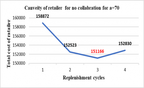
For no collaboration, Table 1, Table 2, Figure 2 and Figure 3 show optimal retailer’s overall cost for a= 40,50,60,70,80 are \$124188, \$135541, \$144159, \$151166 and $158282 are reach its minimum at 7, 8, 8 and 8 optimal ordering cycles respectively. After reaching its minimum at n1=7, 7, 8, 8 and 8 then again started increasing gradually for all upcoming cycles. Table 1 shows the convexity of the retailer’s cost.
This is also discussed in this section with the help of graphical illustrations.
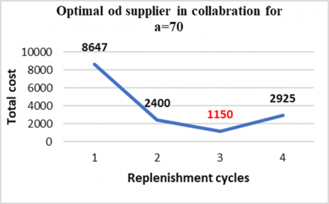
In the case of collaboration, Table 3, Table 4 and Figure 4 give us the optimal supplier’s overall cost for different value of a= 40, 50, 60, 70, 80 are \$896, \$946, \$1103, \$1150 and \$ at 7, 8, 8 and 8 optimal ordering cycles respectively. Again, after attaining its minimum at n2=7, 7, 8, 8 and 8 then again started increasing gradually for all next upcoming cycles. Table 3, Table 5, Table 6, Figure 2, Figure 3, and Figure 4 provided us with information on convexity whenever supplier and retailer are in with no collaboration and with collaboration.
Table 1. The total cost of the retailer with no collaboration with the supplier for different values of a and n1
|
↓a |
→ n |
1 |
2 |
3 |
4 |
5 |
6 |
7 |
8 |
9 |
|
40 |
1382870 |
367427 |
203246 |
152401 |
132840 |
125552 |
124188 |
126095 |
129983 |
|
|
50 |
160150 |
421552 |
230447 |
170745 |
147239 |
137958 |
135541 |
136910 |
140572 |
|
|
60 |
185790 |
484481 |
260902 |
189908 |
160987 |
148596 |
144179 |
144159 |
146801 |
|
|
70 |
2107720 |
545702 |
290439 |
208455 |
174276 |
158872 |
152523 |
151166 |
152830 |
|
|
80 |
2359060 |
607653 |
320403 |
227303 |
187791 |
169324 |
161006 |
158282 |
158945 |
|
Table 2. Optimal retailer’s cost and optimal replenishment cycles with no collaboration different value of a and n1
|
↓a |
→ ti |
t0 |
t1 |
t2 |
t3 |
t4 |
t5 |
t6 |
t7 |
t8 |
t9 |
$T_{I N D}^r$ |
|
40 |
0 |
0.5688 |
1.1105 |
1.6303 |
2.1318 |
2.6177 |
3.0900 |
3.5503 |
4. |
|
124188 |
|
|
50 |
0 |
0.5590 |
1.0957 |
1.6138 |
2.1158 |
2.6040 |
3.0799 |
3.5449 |
4. |
|
135541 |
|
|
60 |
0 |
0.4939 |
0.9717 |
1.4354 |
1.8869 |
2.3274 |
2.7581 |
3.1799 |
3.5937 |
4. |
144159 |
|
|
70 |
0 |
0.4884 |
0.9628 |
1.4249 |
1.8760 |
2.3173 |
2.7496 |
3.1737 |
3.5903 |
4. |
151166 |
|
|
80 |
0 |
0.4840 |
0.9557 |
1.4164 |
1.86721 |
2.3090 |
2.74255 |
3.16854 |
3.58752 |
4. |
158282 |
|
Table 3. The total cost of the supplier in the case of collaboration for different values of a and n2
|
↓a |
→n2 |
1 |
2 |
3 |
4 |
5 |
6 |
7 |
8 |
9 |
|
40 |
1259810 |
243811 |
79609 |
28827 |
9359351 |
2159 |
896 |
2906 |
6900 |
|
|
50 |
1467320 |
286674 |
95520 |
35871 |
12449 |
3263 |
946 |
2420 |
6189 |
|
|
60 |
1715340 |
341075 |
117420 |
46470 |
17629 |
5332 |
1017 |
1103 |
3854 |
|
|
70 |
1958350 |
395364 |
140004 |
58057 |
23956 |
8647 |
2400 |
1150 |
2925 |
|
|
80 |
2202780 |
450279 |
162908 |
69839 |
3040 |
12029 |
3815 |
1200 |
1974 |
|
Table 4. Optimal supplier’s cost and optimal replenishment cycles with the collaboration of different values a and n2
|
↓a |
→ti |
t0 |
t1 |
t2 |
t3 |
t4 |
t5 |
t6 |
t7 |
t8 |
t9 |
$T_{J T}^s$ |
|
40 |
0 |
0.5689 |
1.1105 |
1.6303 |
2.1318 |
2.617 |
3.0901 |
3 4 |
4. |
|
896 |
|
|
50 |
0 |
0.5591 |
1.0958 |
1.6138 |
2.1159 |
2.6041 |
3.0800 |
3.5449 |
4. |
|
946 |
|
|
60 |
0 |
0.4940 |
0.9717 |
1.4355 |
1.8869 |
2.3274 |
2.7582 |
3.180 |
3.5937 |
4. |
1103 |
|
|
70 |
0 |
0.4884 |
0.9628 |
1.4250 |
1.8761 |
2.3173 |
2.7496 |
3.1737 |
3.5903 |
4. |
1150 |
|
|
80 |
0 |
0.4840 |
0.9557 |
1.4164 |
1.8672 |
2.309 |
2.7425 |
3.1685 |
3.5875 |
4. |
3815 |
|
Table 5. Optimality with collaboration and without collaboration different values of a and n2
|
|
|
with collaboration without collaboration |
||||||||||
|
Parameters |
$n_1^*$ |
$T_{I N D}^r$ |
$T_{I N D}^s$ |
$Q_{I N D}$ |
$\delta_{\min }$ |
$\delta_{\max }$ |
$n_2^*$ |
$T_{J T}^r$ |
$T_{J T}^s$ |
$Q_{J T}$ |
$\% T_{I N D}^r$ |
$\% T_{I N D}^r$ |
|
40 |
7 |
124188 |
137511 |
1378.8 |
0.00168 |
0.00160 |
7 |
127440 |
140763 |
1378.8 |
2.61 |
2.36 |
|
50 |
7 |
135541 |
172653 |
1580.2 |
0.00171 |
0.00182 |
7 |
130399 |
167512 |
1580.2 |
3.7 |
2.9 |
|
60 |
8 |
144159 |
242246 |
1633.0 |
0.00178 |
0.00234 |
7 |
115525 |
213612 |
1781.3 |
19.8 |
11.8 |
|
70 |
8 |
151166 |
280562 |
1817.2 |
0.00042 |
0.00239 |
8 |
36393 |
165791 |
1817.2 |
75.9 |
40.9 |
|
80 |
8 |
158282 |
320269 |
2001.2 |
0.00043 |
0.00252 |
8 |
26203 |
188190 |
2001.2 |
83.4 |
41.2 |
Table 6. Sensitivity findings and analysis by variation in different parameters
|
%Change in Parameters |
a |
b |
$\theta$ |
$O_r$ |
CO2 |
A |
$S_s$ |
α |
$h_c$ |
$\tau$ |
$W_p$ |
|
|
$\frac{\triangleleft \overline{T c}_r^{C \rho}}{\overline{T c}_{r o}^{C \rho}} \times 100 \%$ |
$\left\{\begin{array}{c}-20 \\ -10 \\ 0 \\ +10 \\ +20\end{array}\right.$ |
120.938 104.812 70.0103 35.064 0. |
-5.994 -1.773 -1.155 -0.564 0. |
-24.794 -12.177 -9.003 -1.275 0. |
-0.164 0. 0. 0. 0. |
2.555 0. 0. 0. 0. |
-18.833 -10.473 -10.712 -5.429 0. |
-3.485 0.078 0.052 0.026 0. |
-13.135 -6.790 -8.579 -4.482 0. |
0.205 0.153 0.102 0.051 0. |
-3.215 0.311 0.207 0.103 0. |
-4.340 -0.574 -0.383 -0.191 0. |
|
$\frac{\triangleleft \overline{T c}_s^{c_\rho}}{\overline{T c}_{s o}^{c_\rho}} \times 100 \%$ |
$\left\{\begin{array}{c}-20 \\ -10 \\ 0 \\ +10 \\ +20\end{array}\right.$ |
-32.186 -24.402 -16.274 -8.139 0. |
-18.438 -15.536 -10.412 -5.232 0. |
-878.38 -1140.69 -501.20 -616.63 0. |
-5.142 0. 0. 0. 0. |
7.392 0. 0. 0. 0. |
115.770 144.072 -21.002 -10.644 0. |
2.245 -0.596 -0.397 -0.198 0. |
176.399 193.323 -16.307 -8.520 0. |
-0.174 -0.130 -0.087 -0.043 0. |
2.677 -0.259 -0.172 -0.086 0. |
1.471 -1.168 -0.778 -0.389 0. |
|
$\frac{\triangleleft \bar{\delta}}{\bar{\delta}_0} \times 100 \%$ |
$\left\{\begin{array}{c}-20 \\ -10 \\ 0 \\ +10 \\ +20\end{array}\right.$ |
-15.196 -11.028 -6.945 -3.290 0. |
-4.162 -4.936 -3.216 -1.572 0. |
-38692.43 -20318.62 -2929.29 -1477.71 0. |
-5.204 0. 0. 0. 0. |
7.335 0. 0. 0. 0. |
288.762 277.491 -0.127 -0.057 0. |
2.820 -0.202 -0.134 -0.067 0. |
322.398 309.718 0 0 0 |
-0.176 -0.132 -0.088 -0.044 0. |
2.713 -0.262 -0.175 -0.087 0. |
1.491 -1.184 -0.789 -0.394 0. |
|
$n_1^*$ |
$\left\{\begin{array}{c}-20 \\ -10 \\ 0 \\ +10 \\ +20\end{array}\right.$ |
8 8 8 8 8 |
8 8 8 8 8 |
7 7 8 8 9 |
8 8 8 8 8 |
9 9 9 9 9 |
7 7 8 8 8 |
8 8 8 8 8 |
7 7 8 8 8 |
8 8 8 8 8 |
8 8 8 8 8 |
8 8 8 8 8 |
|
$n_2^*$ |
$\left\{\begin{array}{c}-20 \\ -10 \\ 0 \\ +10 \\ +20\end{array}\right.$ |
8 8 8 8 8 |
8 8 8 8 8 |
7 7 8 8 9 |
8 8 8 8 8 |
9 9 9 9 9 |
7 7 8 8 8 |
8 8 8 8 8 |
7 7 8 8 8 |
8 8 8 8 8 |
8 8 8 8 8 |
8 8 8 8 8 |
Figure 2. Pictorial presentation for Table 1
Figure 3. Convexity representation for Table 1
Figure 4. Pictorial presentation for Table 3
The level of sensitivity of each parameter in the Example is illustrated in Table 6. Sensitivity findings and analysis were attained by varying the value of each component that is used in the Example by $-10 \%,-20 \%, 20 \%$, and $10 \%$. As all of us fully understand, the lack of certainty and the unpredictable nature of real economic conditions can cause fluctuation in the values of some variables in a decision-making scenario. Therefore, it's indeed essential to examine the resulting changes besides altering the different parameters. This seems to be possible through comprehensive sensitivity analysis, which illustrates the effects of altering variables. Each of the parameters $O_r$, $h_c$, $\Theta$, $W_p$, $\mathrm{a}$, $\mathrm{b}$, $S_s$, $\hat{c}$, $\hat{P}_r$, $\mathrm{Co}_2$, $\tau$, $C_p$, $\delta$, $\alpha$, $\mathrm{v}_{\mathrm{c}}$, $\mathrm{e}_2$, $\mathrm{e}_1$, $\mathrm{C}_1$, $\mathrm{C}_2$, $\mathrm{~d}$, $\mathrm{~F}_{\mathrm{c}}$, $\mathrm{A}$, $\mathrm{T}$, and $\mathrm{h}$ are changed one by one %. Only one parameter value is changeable slightly at a time remains the parameters keep fixed. Sensitivity Analysis and observations for $\overline{T c}_r^{C \rho}$, $\overline{T c}_s^{C \rho}$, $\bar{\delta}$, $\mathrm{n} 1 *$ and $\mathrm{n} 2 *$ by $-10 \%,-20 \%$, $+20 \%$, and $+10 \%$, concentrating attention on one component at a time and keeping the remaining values fixed. This process of observation was completed with the succour of "MATHEMATICA" numerical iterative computation application version-12. This is analysed in detail by using Table 6. As a result of the study, the value of $n 1^*$ and $n 2^*$ is shown in Table 6 to be highly reactive for the parameters like A, $\alpha$, and, $\Theta$ and insensitive to other left parameters such as $S_s, \mathrm{Co}_2, \tau, C_p, O_r, h_c, W_p, \mathrm{a}$, and $\mathrm{b}$.
1. The average credit $\bar{\delta}$ given by the supplier to the retailer is very sensitive to the parameters $\Theta$, and $A$, moderately sensitive to $\tau, h_c$, and practically insensitive to $S_s, \mathrm{Co}_2, C_p, O_r, W_p$, and b.
2. The total cost of the retailer's $\overline{T c}_r^{C_\rho}$ is very sensitive to the parameters, a and $A$, moderately sensitive to $\Theta$ and practically insensitive to $S_s, \mathrm{Co}_2, \tau, C_p, O_r, h_c, W_p$, and b.
3. The total cost of the supplier's $\overline{T c} c_s^{C \rho}$ is very sensitive to the parameters, a, $\Theta$, and A. moderately sensitive to $S_s, \tau, C_p, h_c, W_p$, and b. and practically insensitive to $\mathrm{Co}_2$, and $\mathrm{O}_r$.
We can apply the findings of this article in a variety of ways to build better deals. First, we can illustrate our approach to determining effective terms such as time, and no. of items and advertisement of new launched or carbon-free products, and conditions in existing markets. Second, manufacturers can make better use of their current resources by making a major contribution to a more sustainable environment (Table 6) by lowering carbon emissions caused by the manufacturing process, supply, or service based on the availability of carbon footprint measurements and identified analysis. They can determine how much of each product to generate to keep inside a GHG emissions cap decided by the government or some regulatory (policy-making) agencies. Third, producers can do a sensitivity analysis to evaluate the optimum cost (Figure 2) of a product enhancement to the long-term profit obtained from that investment. This information will also help manufacturers to reduce costs, manage and control inventory, enhance working capacity and increase customer demand for their products. Moreover, this research increases flexibility throughout the manufacturing process, leading to better resource usage and, as a result, the possibility of increased profit.
This article introduces an optimization technique for identifying the optimal ordering replenishment policies for supply chain management with time, carbon, and advertisement demands. The framework includes an optimization module that is based on an algorithm with and without coordination. A single retailer and supplier with a single-item chain system were thoroughly examined in this study. To best our research knowledge, this is the first study of both centralized and decentralized controls for an inventory system using an advertisement demand-based optimization setting.in collaboration cases, the supplier's main purpose reduces their cost provide. Therefore, credit is offered by the supplier to the retailer. As a result of collaboration, the total cost of both suppliers as well as retailers has been reduced than without collaboration.
To avoid the complexity of the model, we have limited consideration of single supplier-retailer collaboration for a single item with no shortages. But in future, we will extend this by adding some extra parameters, such as multi-echelon, and carbon offset. it also can be developed by taking shortages in the future. In Future, this research study may look into the multi-item and multi-echelon models with time, inventory, and advertising-dependent demand. Some other logical extension is the reworking process during the production of the defective item.
[1] Kaya, Y. (1989). Impact of carbon dioxide emission control on GNP growth: interpretation of proposed scenarios. Intergovernmental Panel on Climate Change/Response Strategies Working Group, May.
[2] Khan, M.A.A., Shaikh, A.A., Konstantaras, I., Bhunia, A.K., Cárdenas-Barrón, L.E. (2020). Inventory models for perishable items with advanced payment, linearly time-dependent holding cost and demand dependent on advertisement and selling price. International Journal of Production Economics, 230: 107804. https://doi.org/10.1016/j.ijpe.2020.107804
[3] Zhou, X., Wei, X., Lin, J., Tian, X., Lev, B., Wang, S. (2021). Supply chain management under carbon taxes: A review and bibliometric analysis. Omega, 98: 102295. https://doi.org/10.1016/j.omega.2020.102295
[4] Liu, Z.L., Anderson, T.D., Cruz, J.M. (2012). Consumer environmental awareness and competition in two-stage supply chains. European Journal of Operational Research, 218(3): 602-613. https://doi.org/10.1016/j.ejor.2011.11.027
[5] Benjaafar, S., Li, Y., Daskin, M. (2012). Carbon footprint and the management of supply chains: Insights from simple models. IEEE Transactions on Automation Science and Engineering, 10(1): 99-116. https://doi.org/10.1109/TASE.2012.2203304
[6] Cheng, Y., Mu, D., Zhang, Y. (2017). Mixed carbon policies based on cooperation of carbon emission reduction in supply chain. Discrete Dynamics in Nature and Society, 2017: 4379124. https://doi.org/10.1155/2017/4379124
[7] Park, S.J., Cachon, G.P., Lai, G., Seshadri, S. (2015). Supply chain design and carbon penalty: Monopoly vs. monopolistic competition. Production and Operations Management, 24(9): 1494-1508. https://doi.org/10.1111/poms.12373
[8] Goyal, S.K., Gunasekaran, A. (1995). An integrated production-inventory-marketing model for deteriorating items. Computers & Industrial Engineering, 28(4): 755-762. https://doi.org/10.1016/0360-8352(95)00016-T
[9] Bhunia, A.K., Maiti, M. (1997). An inventory model for decaying items with selling price, frequency of advertisement and linearly time-dependent demand with shortages. IAPQR Transactions, 22: 41-50.
[10] Shah, N.H., Pandey, P. (2009). Deteriorating inventory model when demand depends on advertisement and stock display. International Journal of Operations Research, 6(2): 33-44.
[11] Bhunia, A.K., Shaikh, A.A. (2011). A two warehouse inventory model for deteriorating items with time dependent partial backlogging and variable demand dependent on marketing strategy and time. International Journal of Inventory Control and Management, 1(2): 95-110.
[12] Shah, N.H., Soni, H.N., Patel, K.A. (2013). Optimizing inventory and marketing policy for non-instantaneous deteriorating items with generalized type deterioration and holding cost rates. Omega, 41(2): 421-430. https://doi.org/10.1016/j.omega.2012.03.002
[13] Bhunia, A., Shaikh, A. (2014). A deterministic inventory model for deteriorating items with selling price dependent demand and three-parameter Weibull distributed deterioration. International Journal of Industrial Engineering Computations, 5(3): 497-510. http://dx.doi.org/10.5267/j.ijiec.2014.2.002
[14] Shaikh, A.A., Mashud, A.H.M., Uddin, M.S., Khan, M. A.A. (2017). Non-instantaneous deterioration inventory model with price and stock dependent demand for fully backlogged shortages under inflation. International Journal of Business Forecasting and Marketing Intelligence, 3(2): 152-164. https://doi.org/10.1504/IJBFMI.2017.084055
[15] Mishra, U. (2018). Optimizing a three-rates-of-production inventory model under market selling price and advertising cost with deteriorating items. International Journal of Management Science and Engineering Management, 13(4): 295-305. https://doi.org/10.1080/17509653.2018.1445046
[16] Panda, G.C., Khan, M.A.A., Shaikh, A.A. (2019). A credit policy approach in a two-warehouse inventory model for deteriorating items with price-and stock-dependent demand under partial backlogging. Journal of Industrial Engineering International, 15(1): 147-170. https://doi.org/10.1007/s40092-018-0269-3
[17] Wu, C., Zhao, Q. (2014). Supplier-retailer inventory coordination with credit term for inventory-dependent and linear-trend demand. International Transactions in Operational Research, 21(5): 797-818. https://doi.org/10.1111/itor.12060
[18] Singh, P., Mishra, N.K., Singh, V., Saxena, S. (2017). An EOQ model of time quadratic and inventory-dependent demand for deteriorated items with partially backlogged shortages under trade credit. In AIP Conference Proceedings, 1860(1): 020037. https://doi.org/10.1063/1.4990336
[19] Kim, S.J., Sarkar, B. (2017). Supply chain model with stochastic lead time, trade-credit financing, and transportation discounts. Mathematical Problems in Engineering, 2017: 6465912. https://doi.org/10.1155/2017/6465912
[20] Barman, A., Das, R., De, P.K. (2020). Pricing and inventory decisions of multi-item deteriorating inventory system under stock, time and price sensitive demand policy. In 2020 9th International Conference System Modeling and Advancement in Research Trends (SMART), pp. 453-458. https://doi.org/10.1109/SMART50582.2020.9337124
[21] Daryanto, Y., Wee, H.M., Astanti, R.D. (2019). Three-echelon supply chain model considering carbon emission and item deterioration. Transportation Research Part E: Logistics and Transportation Review, 122: 368-383. https://doi.org/10.1016/j.tre.2018.12.014
[22] Xiang, D., Lawley, C. (2019). The impact of British Columbia's carbon tax on residential natural gas consumption. Energy Economics, 80: 206-218. https://doi.org/10.1016/j.eneco.2018.12.004
[23] Shi, Y., Zhang, Z., Chen, S.C., Cárdenas-Barrón, L.E., Skouri, K. (2020). Optimal replenishment decisions for perishable products under cash, advance, and credit payments considering carbon tax regulations. International Journal of Production Economics, 223: 107514. https://doi.org/10.1016/j.ijpe.2019.09.035
[24] Mishra, N.K., Ranu. (2022). A supply chain inventory model for deteriorating products with carbon emission-dependent demand, advanced payment, carbon tax and cap policy. Mathematical Modelling of Engineering Problems, 9(3): 615-627. https://doi.org/10.18280/mmep.090308
[25] Sarkar, T., Ghosh, S.K., Chaudhuri, K. (2012). An optimal inventory replenishment policy for a deteriorating item with time-quadratic demand and time-dependent partial backlogging with shortages in all cycles. Applied Mathematics and Computation, 218(18): 9147-9155. https://doi.org/10.1016/j.amc.2012.02.072