Duaa M. Rasol* | Salah R. Al-Zaidee
© 2022 IIETA. This article is published by IIETA and is licensed under the CC BY 4.0 license (http://creativecommons.org/licenses/by/4.0/).
OPEN ACCESS
This study aims to investigate the dynamic Load allowance variation (DLA) of dynamic tank Loads and compare it with Iraq's standard specifications for road bridges. DLA is considered a simple measurement of the dynamic variation magnitude of the tank load for a specific combination of road roughness and speed. In addition to determining the stochastic dynamic response of the bridge. Al-Awsej bridge in Iraq, with a span of 33.2 m and a principal road with four pavement roughness classes (very good, good, average, and poor), was proposed as a case study in this analysis. A spectral closed-form solution was used for evaluating the dynamic tank load due to the passage of a tank type-72A at a constant speed of 40,50,60 and 70 km/hr along a bridge with different types of rough pavement surface. The results show the less value of DLA for very good pavement at 40 km/hr is about 0.032, and the largest value is about 0.293 at 70 km/hr for poor pavement. Also, road surface roughness greatly influences vehicle-bridge interactions and bridge responses. Where at 40 km/hr, the Root mean square of bridge deflection range from 0.31 to 2.75 mm and 0.39 to 3.14 mm at 70 km/hr.
dynamic tank load, pavement roughness, dynamic load allowance, bridge, modal analysis, dynamic response of a bridge
The dynamic force generated by the interaction of the bridge caused by the passage of vehicles plays an important role in the design of the bridge structure. In practice, usually, a moving static load is used to model the vehicle force on bridges, and the static design loads are increased by a dynamic load allowance (DLA) to account for the dynamic effects from the vehicle vibrations due to the interaction between the vehicle and bridge [1].
Many codes specify the DLA as a function of span length only which might not lead to a reliable prediction of the dynamic loads on the bridge due to avoiding dynamic response analysis of the vehicle vibration that is moving along the bridge allow for a straightforward estimation of the vehicle loads in the bridge design [2]. The dynamic load that is caused by the interaction between the vehicle and the bridge is a difficult problem that is impacted by a wide variety of parameters including, the level of roughness of the road surface, the speed of the vehicle, and the dynamic properties of both the vehicle and the bridge. Therefore, there has been an increasing interest in and concern about bridge design forces [3].
Thus, determining the vehicle's dynamic load due to the vehicle's passage through the span of the bridge is a problem of great interest to bridge engineers. Therefore, an approach was developed, and a simple closed-form solution was derived to predict a vehicle's dynamic load for bridge design applications. Two sets of equations of motion were written to solve the problem of vehicle-bridge interaction, one for the vehicle and the other for the bridge, and in order to mathematically relate the motion of the vehicle and the bridge, the interactive force existing at the contact point between the vehicle and bridge is considered [4, 5].
In this study, numerical analysis has been carried out to calculate the dynamic load allowance and the stochastic response of the bridge because of the passage of a vehicle moving at constant speed along a rough bridge surface. The vehicle has been replaced by a simple, linear, damped spring-mass system which moves on a bridge at a constant speed. The bridge has been represented as simply support with a single degree of freedom.
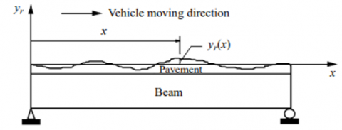
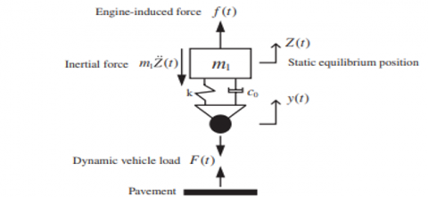
In this study, the vehicle is modeled as a single degree of freedom (SDOF) with mass m1, constant spring k, and damping coefficient c0 with constant speed V along a rough bridge pavement (see Figure 1 (a)). A possible profile of the irregularities of pavement surface on a bridge, as shown in Figure 1 (b), the height, yr of the surface is plotted as a function of distance x along the bridge [3, 5]. The pavement-surface elevation $\tilde{y}(d, t)$ represent the sum of the pavement roughness and displacement of the bridge. The equation of motion of the vehicle is given by:
$m_1 \ddot{\tilde{z}}(t)+c_0\left(\dot{\tilde{z}}(t)-\hat{y}_{x=d}\right)+k\left(\tilde{z}(t)-\tilde{y}_{x=d}\right)$$=f(t)-m_1 g$ (1)
where, $\ddot{\tilde{z}}$, $\dot{\tilde{z}}$, and $\tilde{Z}$ are absolute acceleration, velocity, and displacement of the vehicle, respectively. f(t) and m1g are the engine-induced force and the vehicle gravity force, respectively. The d=Vt expresses the moving distance of the vehicle on the bridge. Rearranging Eq. (1) to become:
$m_1 \ddot{\tilde{z}}(t)+c_0 \dot{\tilde{z}}(t)+k \tilde{z}(t)$$\quad=f(t)-m_1 g+c_0 \tilde{y}_{x=d}+k \tilde{y}_{x=d}$ (2)
Since y(x, t)=y(x=d=Vt, t), Eq. (2) reductions into the typical form of a linear SDOF system. The time-varying parameter y(d, t), the engine-induced force f(t), and the vehicle gravity force m1g are all inputs to the suspension system. Note that y(d, t) may be represented as the sum of the bridge deflection $y_b(d, t)$ due to moving vehicle gravity force (a constant moving force), the bridge deflection yb(d, t) due to moving random dynamic vehicle load F(t), and the pavement roughness yr(t). Let:
$\tilde{Z}(t)=Z_1(t)+Z(t)$ (3)
$\tilde{y}(d, t)=y_{b_1}(d, t)+y_r(t)+y_b(d, t)$ (4)
and
$y(d, t)=y_r(t)+y_b(d, t)$ (5)
Eq. (2) is divided into two equations:
$m_1 \ddot{z}_1(t)+c_0 \dot{z}_1(t)+k z_1(t)$$=c_0 \dot{y}_{b_1}(d, t)+k y_{b_1}(d, t)$ (6)
$m_1 \ddot{z}(t)+c_0 \dot{z}(t)+k z(t)$$\quad=f(t)-m_1 g+c_0 \dot{y}(d, t)$$\quad+k y(d, t)$ (7)
where, $y_{b_1}(d, t)$ is the bridge deflection as a result of the constant moving force m1g and the vehicle displacement z1(t) in Eq. (6) are deterministic functions; f(t), y(d, t), and Z(t) in Eq. (7) are random functions. If $y_{b_1}(d, t)$ is known, z1(t) of Eq. (6) can be easily resolved using any available methods [6, 7].
(a)
(b)
(c)
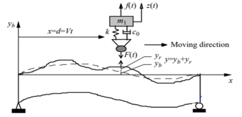
Figure 1. (a) Road roughness profile, (b) Vehicle model, (c) Bridge model subjected to dynamic vehicle load [6]
Suppose a vehicle's equation of motion is expressed in the static-equilibrium position. In that case, it will be referenced to the vehicle's displacements in future discussions when the vehicle's dynamic "random" response will be calculated [1, 8]. The analytical model of the dynamic vehicle-bridge interactive system is shown in Figure 1 (c). The total response of the vehicle, such as spring force, displacement, etc., is achieved by including the static response to the dynamic analysis results. The static responses that cause by gravity force from vehicle weight. The static force of the vehicle also represents the mean of the stochastic load, and it's considered the reference position when the system vibrates. Then to study the dynamic response separately from the static, the static force was ignored when considering the zero mean gaussian process. Then, Eq. (7) becomes [9]:
$m_1 \ddot{z}(t)+c_0 \dot{z}(t)+k z(t)=f(t)+c_0 \dot{y}(d, t)+k y(d, t)$ (8)
If y(d, t) and f(t) have, respectively, power spectral density function Syy(d, ω) and Sff(ω) with respect to time, the relation of the power spectral density function of the vehicle response Szz(d, ω) and of the inputs is then given by:
$S_{z z}(d, \omega)=\sum_r \sum_s H_r{ }^*(\omega) H_s{ }^*(\omega) S_{r s}(d, \omega)$$r, s=y(d, t), f(t)$ (9)
where, $H_r{ }^*(\omega)$ is the complex conjugate of Hr(ω).
In general, the engine-induced force f(t) exhibits a harmonic form and little correlative with the pavement roughness and the moving distance of a vehicle. For uncorrelated inputs, Szz (d, ω) can be expressed by the relation:
$S_{z z}(d, \omega)=\left|H_y(\omega)\right|^2 S_{y y}(d, \omega)+\left|H_f(\omega)\right|^2 S_{f f}(\omega)$ (10)
where,
$H_y(\omega)=\frac{k+i c_0 \omega}{\left(k-m_1 \omega^2\right)+i c_0 \omega}$ (11)
and
$H_f(\omega)=\frac{1}{\left(k-m_1 \omega^2\right)+i c_0 \omega}$ (12)
If the influence of engine motion on vehicle vibration is ignored as in this study, the Szz (d, ω) become:
$S_{z z}(d, \omega)=\left|H_y(\omega)\right|^2 S_{y y}(d, \omega)$ (13)
The degree of unevenness of the road surface is the most important component that determines the dynamic load allowance for the bridge design [10]. In most cases, the method of variation of a bridge surface as a distance function is considered to be a zero-mean stationary random process. During the earlier stages of pavement roughness characterization, this assumption of Gaussian was prevalent and was based on numerous and extensive pavement profile surveys undertaken across the world that have shown that pavement profiles can be considered random with an approximately zero-mean stationary Gaussian probability distribution. The power spectral density is a function of yr m2⁄(cycle⁄m) and it is approximated by Eq. (14) [11]:
$S_{y_r y_r}(\omega)$$=\left\{\begin{array}{ll}\frac{1}{2 \pi V} S\left(n_0\right)\left(\frac{\omega}{2 \pi V n_0}\right)^{-\omega_1}, & \omega \leq 2 \pi V n_0 \\ \frac{1}{2 \pi V} S\left(n_0\right)\left(\frac{\omega}{2 \pi V n_0}\right)^{-\omega_2}, & \omega>2 \pi V n_0\end{array}\right\}$ (14)
where, n is the spatial frequency or wave number (cycle/m), which expresses the rate of change with respect to distance, and it is a function of wavelength Lw. S(n0) is the pavement roughness coefficient (m3/cycle). n0, discontinuity frequency (cycle/m) is the reference spatial frequency, ω1, and ω2 are the parameters of spectral shape. V is the vehicle speed and the time angular frequency ω by (rad/sec) expressed [12, 13]:
$\omega=2 \pi n V$ (15)
The parametric values for typical principal roads as shown in Table 1.
Table 1. Pavement classes are based on principal roads [14]
|
Pavement class |
$S\left(n_0\right)$ $\frac{m^3}{\text { cycle }}$ |
ω1 |
ω1 |
||
|
Mean |
Standard deviation |
Mean |
Standard deviation |
||
|
Very good |
2×10⁻⁶ |
2.05 |
0.487 |
1.44 |
0.266 |
|
Good |
8×10⁻⁶ |
||||
|
Average |
32×10-6 |
||||
|
Poor |
128×10-6 |
||||
The dynamic vehicle load F(t) is calculated empirically for a specific stretch of pavement, and it is supposed to have the properties of a stationary Gaussian random process with zero mean value. Considering that the power spectral density function was used to characterize the F(t), and that the F(t) is defined [15]:
$F(t)=C_0(\dot{Z}-\dot{y})+k(Z-y)=f(t)-m_1 \ddot{Z}$ (16)
The spectral density function of F(t) is approximately given by Eq. (17):
$S_{F F}(\omega)=T_f(\omega) S_{f f}(\omega)+T_r(\omega) S_{y_r y_r}(\omega)$ (17)
The Tf and Tr are expressed by Eq. (18) and Eq. (19), respectively:
$T_f(\omega)=1+m_1{ }^2 \omega^4\left|H_f(\omega)\right|^2$ (18)
$T_r(\omega)=m_1^2 \omega^4\left|H_y(\omega)\right|^2$ (19)
Then, the mean square and Root mean square of F(t) is related to SFF(ω) by Eq. (20), and Eq. (21), respectively:
$\sigma_F^2=\int_0^{\infty} S_{F F}(\omega) d \omega$ (20)
$\sigma_F=\sqrt{\sigma_F^2}$ (21)
The DLA is a significant design and assessment parameter. The magnitude of the dynamic load allowance, which is determined by Eq. (22), depends on the bridge's vibrations, the roughness of the pavement, the vehicle's speed, and the vehicle's suspension system [5]. Hence, the wavelength is considered a function of spatial frequency n and the spatial frequency converts to cyclic or circular frequency ω through Eq. (15); one of the most essential variables in this equation is vehicle speed because it can increase the frequency range of the load when increasing the vehicle speed.
$D L A=\frac{\sigma_F}{m_1 g}$ (22)
7.1 Equation of motion of bridge
The transverse deflection yb (x, t) of the bridge at time t and distance x satisfies the partial differential equation given by Eq. (23) because the bridge with length L and mass per unit length $\bar{m}$ is elastic uniform straight and subjected to a viscous damping force c per unit length per unit velocity and a transverse force p(x, t) per unit length [1, 16].
$\bar{m} \frac{\partial^2 \tilde{y}_b}{\partial t^2}+c \frac{\partial \tilde{y}_b}{\partial t}+E I \frac{\partial^4 \tilde{y}_b}{\partial x^4}=p(x, t)$ (23)
where, EI is the constant bending stiffness of the bridge. $p(x, t)$ replaced by Eq. (26) for constant vehicle speed [17].
$p(x, t)=\delta(x-d) p(t)=\delta(x-d)\left(m_1 g+F(t)\right)$$=\delta(x-d) m_1 g+\delta(x-d) F(t)$ (24)
where, $\delta(\cdot)$ is the Dirac distribution, $F(t)$ is a stationary Gaussian random process with zero mean; m1g is the vehicle gravity; the total vehicle load on the bridge P(t) is a stationary Gaussian random process with a mean value of m1g. If F(t) assumed is independent of the mean deterministic deflection of the bridge. Eq. (23) is written as two separate equations as follows:
$\bar{m} \frac{\partial^2 y_{b_1}}{\partial t^2}+c \frac{\partial y_{b_1}}{\partial t}+E I \frac{\partial^4 y_{b_1}}{\partial x^4}=\delta(x-d) m_1 g$ (25)
$\bar{m} \frac{\partial^2 y_b}{\partial t^2}+c \frac{\partial y_b}{\partial t}+E I \frac{\partial^4 y_b}{\partial x^4}=\delta(x-d) F(t)$ (26)
Eq. (25) for deterministic mean values of random function yb(x, t), and p(x, t). while the second, Eq. (26), is valid for their centered "random" components. The total deflection $\tilde{y}_b(x, t)$ of the bridge due to the moving vehicle is the sum of the deflection $y_{b_1}$ of the bridge subject to the constant force $m_1 g$ and the deflection yb due to dynamic vehicle load F(t) (see Figure 1 (c)). $y_b=y_{b_1}+y_b, y_{b_1}$ is a deterministic function, and yb is a random function.
7.2 Response of bridge to dynamic vehicle load
The statistical properties of the second-order (variation of $y_b$) that can be derived from Eq. (26) [1, 18]. One form of a solution of Eq. (26) obtained by separation of variables, assuming that the solution has the form:
$y_b(x, t)=\sum_{i=1}^{\infty} \psi_j(x) Y_j(t)$ (27)
It is believed that the free-vibration motions consist of a series of constant shapes ψj(x), and that the amplitude of these motions varies with time by Yj(t). When analyzing undamped free vibration, it is possible to estimate the undamped angular frequencies readily ωj of the bridge as well as the mode shapes ψj(x) of the bridge by considering the boundary conditions at the ends of the bridge segment. The ωj and ψj(x) values of the bridge can be calculated as follows for a simply supported bridge:
$\omega_j=\left(j \frac{\pi}{L}\right)^2 \sqrt{\frac{E I}{\bar{m}}}$ (28)
or
$f_j=\left(j \frac{\pi}{2 L^2}\right) \sqrt{\frac{E I}{m}}$ (29)
and
$\psi_j(x)=\sqrt{2} \sin \left(j \frac{\pi x}{L}\right)$ (30)
The modes ψj(x) satisfy the orthogonal conditions:
$\int_0^L \psi_j(x) \psi_k(x) d x=L \delta_{j k}$ (31)
where, δjk is the Kronecker delta function.
Substituting Eq. (27) into Eq. (26), multiplying through by ψj(x), integrating over $x$, and using the orthogonal conditions, here the ψj(x) is considered a filter to choose the mode required, all mods that are j≠k are disappearing. Hence, transforming from a multi-degree of freedom to a single degree of freedom leads to the uncoupled equation of motion for Yj(t):
$\ddot{Y}_j+\beta \dot{Y}_j+\omega_j^2 Y_j=G_j(t)$ (32)
where,
$\beta_j=\frac{c}{\bar{m}}$ (33)
and
$G_j(t)=\frac{1}{\bar{m} L} \int_0^L \psi_j(x) \delta(x-d) F(t) d x$ (34)
The convolution integral gives the formal solution to Eq. (32):
$Y_j(t)=\int_0^t G_j(t-\theta) h_j(\theta) d \theta$ (35)
where, the impulse response function is:
$h_j(t)=\left\{\frac{e^{-0.5 \beta_j t}}{\omega_j \sqrt{1-\frac{\beta_j^2}{4 \omega_j^2}}} \sin \left(\omega_j \sqrt{1-\frac{\beta_j^2}{4 \omega_j^2}} t\right)\right\}$, t≥0 (36)
Substituting Eq. (34) into Eq. (35), the modal amplitude Yj(t) may then be written as:
$Y_j(t)=\int_0^t \frac{1}{\overline{m L}} \int_0^L \psi_j(x) \delta(x-d) F(t-\theta) d x h_j(\theta) d \theta$$=\frac{\psi_j(d)}{\overline{m L}} \int_0^L F(t-\theta) h_j(\theta) d \theta$ (37)
Thus,yb(x, t) can be obtained in the form:
$y_b(x, t)=\sum_{j=1}^{\infty} \psi_j(x) Y_j(t)$ (38)
$y_b(x, t)=\sum_{j=1}^{\infty} \frac{\psi_j(x) \psi_j(d)}{\overline{m L}} \int_0^t F(t-\theta) h_j(\theta) d \theta$ (39)
In according to random vibration theory, the spectral density function of yb(x, t) give:
$S_{y_b y_b}(x, \omega)=\frac{1}{2 \pi} \int_{-\infty}^{\infty} R_{y_b y_b}(x, \tau) e^{-i \omega \tau} d \tau$ (40)
where,
$R_{y_b y_b}(x, \tau)=E\left[y_b(x, t) y_b(x, t+\tau)\right]$ (41)
The power spectrum density of bridge deflection is given by Eq. (42):
$S_{y_b y_b}(x, \omega)$$=S_{F F}(\omega) \sum_{j=1}^{\infty} \sum_{k=1}^{\infty} \frac{\psi_j(x) \psi_j(d) \psi_k(x) \psi_k(d)}{(\bar{m} L)^2} H_j(\omega) H_k(-\omega)$ (42)
where, SFF (ω) is the power spectral density function of F(t) and Hj(ω) is the transfer function of the bridge.
$H_j(\omega)=\frac{1}{\left(\omega_j^2-\omega^2\right)+i \beta_j \omega}$ (43)
and
$B(x, \omega)$$=\sum_{j=1}^{\infty} \sum_{k=1}^{\infty} \frac{\psi_j(x) \psi_j(d) \psi_k(x) \psi_k(d)}{(\bar{m} L)^2} H_j(\omega) H_k(-\omega)$ (44)
Finally, the power spectrum density for single degree of freedom system of a bridge may be written as:
$S_{y_b y_b}(x, \omega)$$=S_{F F}(\omega) \frac{1}{(\bar{m} L)^2} \frac{1}{\left(\omega_j^2-\omega^2\right)+i 2 \xi \omega_j \omega}$ (45)
In the following, a numerical example is presented and analyzed to evaluate dynamic load allowance and determine the Root mean square of deflection for the Al-Awsej bridge when stochastic responses due to randomness in dynamic tank load are taken into account.
8.1 Description of parameters in the analysis
In this study, tank T-72A has been proposed to evaluate the variation of dynamic vehicle load. The suspension weight, stiffness, and damping of T-72A have been taken at 37430 kg, 3501 kN/m, and 9 percent of the critical damping. The vibration frequency of the tank T-72 system was equal to 9.67 rad/s (1.54 Hz). Four constant speeds along a rough bridge surface have been considered, 40, 50, 60, and 70 km/ hr. Four classes of pavement roughness (very good, good, average, and poor pavements) have been used. The parameters $n_o$, $\omega_1$, and $\omega_2$ are taken as 0.1 (cycle/m), 2.05, and 1.44, respectively. The effect of engine motion on vehicle vibration has been disregarded.
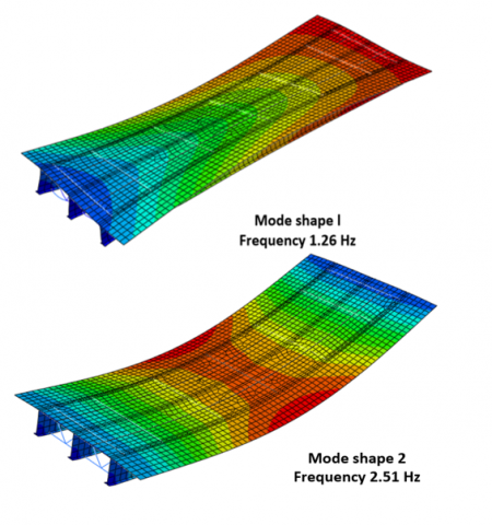
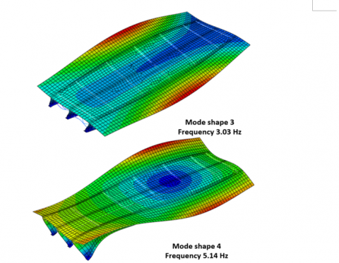
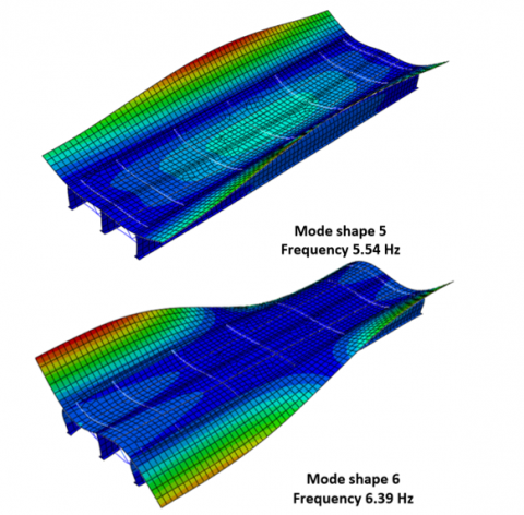
The bridge has been modeled as a simply-supported with a span length of 33.2 m. The mass per unit length m and EI of the bridge were taken as 13761 kg and 33×106 kN.m2, respectively. The modal damping ratio is assumed to be 0.02, and natural frequency was obtained by modal analysis using ABAQUS software. The first six vibration modes are deduced, as shown in Figure 2 and the natural frequency in (Hertz) represented the characteristics of these modes. Rainbow colours represent the mode shapes normalized in such a way to have generalized mass of one unit. The second mode that has been used is equal to 2.51 Hz.
Figure 2. Mode shapes and Frequencies of a bridge
8.2 Results of the analysis
8.2.1 Dynamic vehicle response due to road unevenness
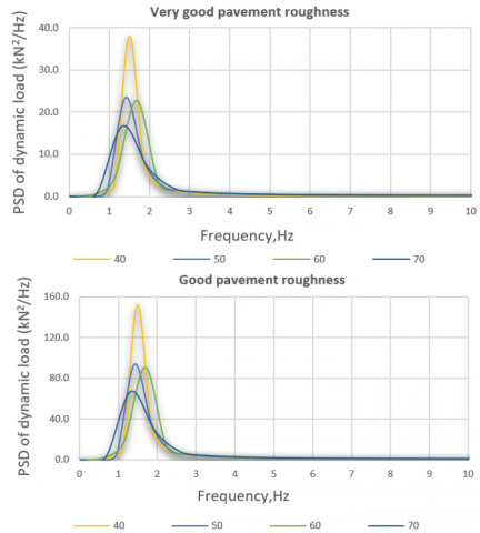
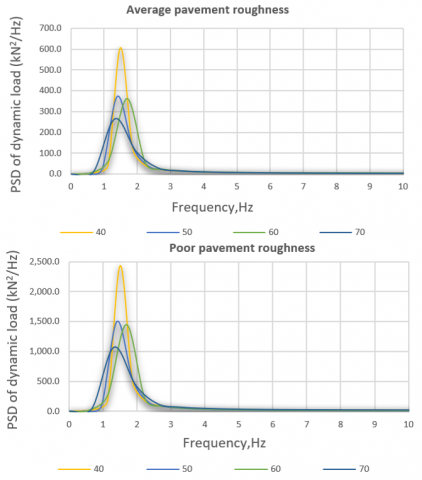
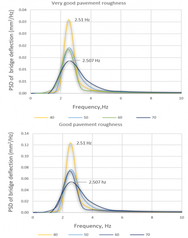
The tank load power spectrum density is deduced from a random process due to pavement roughness which is dependent on the vehicle-pavement coupled model formula.
The power spectrum density (PSD) of the dynamic tank load has been generated for different classes of pavement roughness with a constant speed tank vehicle ranging from 40 to 70 km/hr. The PSD has been presented in Figure 3. The results showed that the peak detected refers to a maximum response that occurs near the frequency of the vehicle.
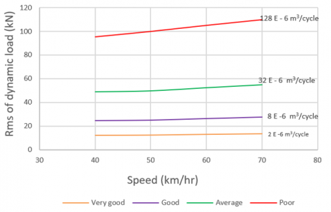
Numerical integration analysis has been performed to deduce the mean square of dynamic tank loads. Consequently, the Root mean square (Rms) of dynamic tank loads has been determined, as shown in Figure 4. It is considered a key feature related to mean energy distribution when the Root mean square formulation translates the power spectral density curve for each response quantity into a single value.
In the case of pavement roughness (very good and good), insignificant effect in Rms of dynamic load with speed increasing. In contrast, in (average and poor) rough pavement conditions, the vehicle speed affects the Rms of dynamic load. At a specified tank speed, the dynamic load increase two times with increased pavement roughness coefficient S(n0) four times. That led to the Rms being proportional to the square Root of the pavement roughness coefficient S(n0).
Figure 3. PSD of dynamic tank load versus tank speed for four classes of pavement roughness
Figure 4. Rms of dynamic tank load for four classes of pavement roughness
8.2.2 Dynamic load allowance
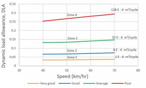
The dynamic load allowance, DLA, has been estimated based on the Rms of dynamic loads achieved in the previous section in Figure 4. the result showed The DLA increases linearly with the increases in vehicle speed and pavement roughness coefficient, as shown in Figure 5.
Figure 5. DLA versus vehicle speed for four classes of pavement roughness
All results of the DLA for various speeds and classes of pavement roughness are illustrated in Table 2, and the result shows the average dynamic load allowance for good and average pavement roughness from 0.068 to 0.137. Generally, most roads belong to these classes, and the DLA of 0.05-0.3 is typical under normal operating conditions and close to zero when the vehicle moves over a perfectly smooth road [19].
Table 2. Dynamic load allowance, DLA
|
Speed (km/hr) |
DLA |
|||
|
Very good |
good |
Average |
Poor |
|
|
40 |
0.032 |
0.065 |
0.130 |
0.252 |
|
50 |
0.033 |
0.066 |
0.133 |
0.267 |
|
60 |
0.035 |
0.070 |
0.140 |
0.280 |
|
70 |
0.036 |
0.073 |
0.146 |
0.293 |
|
Average |
0.034 |
0.068 |
0.137 |
0.273 |
8.2.3 Response bridge
In order to estimate the stochastic response of the bridge due to the dynamic effects of the vehicle vibration when traveling along the bridge resulting from the interaction between the vehicle and bridge, the output power spectrum density of dynamic tank loads at various vehicle speeds and pavement roughness classes will be used as input power spectral density of dynamic load applied on a bridge.
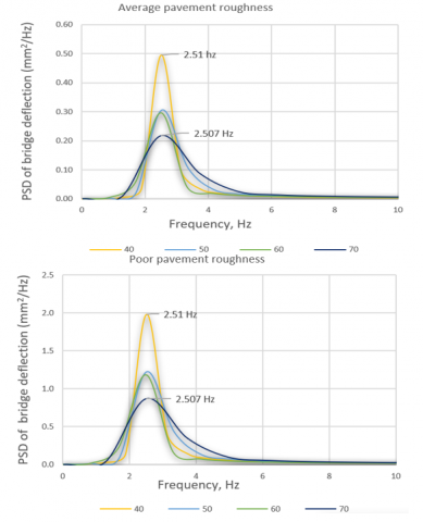
The PSD of bridge deflection has been presented in Figure 6, which is due to more of one realization of the randomly varying road surface roughness, which is sufficient to describe the possible road surface roughness effect on vehicle-bridge interaction. One peak of the PSD of deflection curves can be observed with the increase of the pavement roughness because of the resonance of the coupling system.
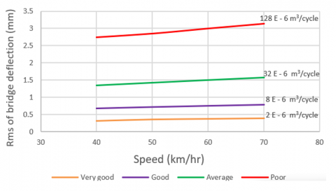
Numerical integration analysis has been performed to deduce the mean square and the Root mean square of bridge deflection, as shown in Figure 7. The increase in the Root mean square of bridge deflection at the vehicle speed (40, 50, 60 and 70) km/hr appears clearly in the case of average and poor roughness pavement. The relationship between the Rms of the bridge deflection and velocity appears to be approximately linear. The underlying reason for this phenomenon is that, at a specified vehicle speed, the Rms of dynamic vehicle load is proportional to the square root of the pavement roughness coefficient S(n0).
Figure 6. PSD of deflection bridge
Figure 7. Rms of bridge deflection
The results of Root mean square of bridge deflection at various speeds and for four classes of roughness pavement (very good, good, average, and poor) are illustrated in Table 3.
Table 3. Rms of bridge deflection for four classes of pavement roughness
|
Speed (km/hr) |
Rms of bridge deflection (mm) |
|||
|
Very good |
Good |
Average |
Poor |
|
|
40 |
0.31 |
0.67 |
1.35 |
2.75 |
|
50 |
0.36 |
0.71 |
1.43 |
2.85 |
|
60 |
0.37 |
0.75 |
1.49 |
2.99 |
|
70 |
0.39 |
0.78 |
1.57 |
3.14 |
A stochastic dynamic analysis of the Al-Awsej bridge has been performed in this paper due to the passage of tank T-72 along a bridge with four classes of pavement surface roughness. The bridge is located in Iraq with a span of 33.2 m. Several vital concepts were presented, including:
·For pavement roughness (very good and good), insignificant effect in Rms of dynamic load with speed increasing. In contrast, in (average and poor) rough pavement conditions, the vehicle speed affects the Rms of dynamic load. At a specified tank speed, the dynamic load increase two times with increased pavement roughness coefficient S(n0) four times. That led to the Rms being proportional to the square root of the pavement roughness coefficient S(n0).
·The dynamic load allowance increases linearly with vehicle speed, and the pavement roughness coefficient increases.
·In the case of the very good pavement roughness surface with increasing vehicle speed, it did not significantly affect the value of the dynamic load allowance. In contrast, in poor rough pavement conditions, the roughness and vehicle speed has significantly affected the dynamic load allowance, where the value approached 0.293 when the vehicle speed approaches 70 km/hr.
·As compared with good and average pavement roughness surface, the dynamic load is still within a limit on Iraq standard specifications for road bridges, while in the case of poor pavement reaches 0.293 at a tank speed of 70 km/hr. So, it can be considered the results of the DLA within the Iraq standard specifications for road bridges because of most roads are classified as good and average pavement roughness.
The road surface roughness greatly influences the vehicle-bridge interactions and dynamic bridge responses at a specified tank speed. At the tank speed of 40 km/hr, the Root mean square of deflection of the bridge increase from 0.31 to 2.75 mm, and at the tank speed of 70 km/hr, the Root mean square of deflection of the bridge increase from 0.39 mm to 3.14 mm.
[1] Lin, J.H., Weng, C.C. (2004). Evaluation of dynamic vehicle load on bridge decks. Journal of the Chinese Institute of Engineers, 27(5): 695-705. https://doi.org/10.1080/02533839.2004.9670917
[2] Ding, L. (2010). Bridge load rating with model updating and stochastic analysis of vehicle-bridge interaction. Doctoral dissertation, University of Western Australia. https://research-repository.uwa.edu.au/files/3229027/Ding_Lina_2010.pdf.
[3] Lin, J.H. (2014). Variations in dynamic vehicle load on road pavement. International Journal of Pavement Engineering, 15(6): 558-563. http://dx.doi.org/10.1080/10298436.2013.770512
[4] Liu, N. (2014). Dynamic analysis of vehicle-bridge interaction system with uncertain parameters. Doctoral dissertation, UNSW Sydney. https://doi.org/10.26190/unsworks/2595
[5] Khavassefat, P. (2014). Vehicle-pavement interaction. Ph.D. Thesis, Royal Institute of Technology, Engineering Sciences, Department of Transport Science, SE-100 44 Stockholm, Sweden. http://orcid.org/0000-0003-2434-6957
[6] Lin, J.H. (2006). Response of a bridge to a moving vehicle load. Canadian Journal of Civil Engineering, 33(1): 49-57. http://dx.doi.org/10.1139/l05-085
[7] Yang, Y.B., Lee, Y.C., Chang, K.C. (2014). Effect of road surface roughness on extraction of bridge frequencies by moving vehicle. In Mechanics and model-based control of advanced engineering systems, pp. 295-305. https://doi.org/10.1007/978-3-7091-1571-832
[8] Lin, J.H., Weng, C.C. (2001). Analytical study of probable peak vehicle load on rigid pavement. Journal of Transportation Engineering, 127(6): 471-476. http://dx.doi.org/10.1061/(ASCE)0733-947X(2001)127:6(471)
[9] Xu, H.L., He, L., An, D. (2017). Study on the vehicle dynamic load considering the vehicle-pavement coupled effect. In IOP Conference Series: Materials Science and Engineering, 269(1): 012001. https://doi.org/10.1088/1757-899X/269/1/012001
[10] Jerath, S. (2015). Road surface roughness generation by power spectral density in bridge design. ASCE. http://dx.doi.org/10.1061/41016(314)312
[11] Dean, A., Martini, R., Brennan, S. (2011). Terrain-based road vehicle localisation using particle filters. Vehicle System Dynamics, 49(8): 1209-1223. https://doi.org/10.1080/00423114.2010.493218
[12] Li, J., Zhang, Z., Gao, X., Wang, P. (2018). Relation between power spectral density of road roughness and international roughness index and its application. International Journal of Vehicle Design, 77(4): 247-271. http://dx.doi.org/10.1504/IJVD.2018.10021450
[13] Camara, A., Vázquez, V.F., Ruiz-Teran, A.M., Paje, S.E. (2017). Influence of the pavement surface on the vibrations induced by heavy traffic in road bridges. Canadian Journal of Civil Engineering, 44(12): 1099-1111. https://doi.org/10.1139/cjce-2017-0310
[14] Lin, J.H., Weng, C.C. (2001). Analytical study of probable peak vehicle load on rigid pavement. Journal of Transportation Engineering, 127(6): 471-476. http://dx.doi.org/10.1061/(ASCE)0733-947X(2001)127:6(471)
[15] Belay, A., OBrien, E., Kroese, D. (2008). Truck fleet model for design and assessment of flexible pavements. Journal of Sound and Vibration, 311(3-5): 1161-1174. http://dx.doi.org/10.1016/j.jsv.2007.10.019
[16] Wei, L., Wang, J., Guo, H., Zhao, Sh., Sun, J. (2020). Dynamic response of latticed shell and its steel column supports under impact load. International Journal of Sustainable Development and Planning, 9(4): 857-861. https://doi.org/10.18280/ijsdp.150217
[17] Li, J., Zhang, H. (2020). Moving load spectrum for analyzing the extreme response of bridge free vibration. Shock and Vibration, 2020. https://doi.org/10.1155/2020/9431620
[18] Jin, Z., Li, G., Pei, S., Liu, H. (2017). Vehicle-induced random vibration of railway bridges: A spectral approach. International Journal of Rail Transportation, 5(4): 191-212. https://doi.org/10.1080/23248378.2017.1338538
[19] Buhari, R., Rohani, M.M., Abdullah, M.E. (2013). Dynamic load coefficient of tyre forces from truck axles. In Applied Mechanics and Materials, 405: 1900-1911. https://doi.org/10.4028/www.scientific.net/AMM.405-408.1900