Syaharuddin | Fatmawati* | Herry Suprajitno
© 2022 IIETA. This article is published by IIETA and is licensed under the CC BY 4.0 license (http://creativecommons.org/licenses/by/4.0/).
OPEN ACCESS
Artificial Neural Networks are widely used in prediction activities and classification processes. However, the implementation on average only uses a network architecture with one hidden layer, while the development of architectures with two or three hidden layers has not been done much. This article discusses the process of developing ANN Backpropagation using a Matlab-based graphical user interface with three hidden layers combined with non-linear activation functions (logsig, tansig, tanh) and training functions (trainrp and trainlm) based on learning rate and momentum. Architecture was created to study climate change in the area around Lombok International Airport station by training on hydrological data (rainfall) from January 2012 to December 2021 with a data type of 10-day interval (36 data every year). The number of neurons in the first hidden layer was determined using the Hecht-Nielsen model, while the second and third hidden layers used the Lawrence-Fredrickson model. Simulation results with architecture 36-73-37-19-1, a learning rate of 0.1, and momentum of 0.9 showed that variations in the activation function logsig-logsig-logsig-purelin and trainlm function demonstrated the best result with epoch of 7, MSE of 0.00090, and RMSE of 0.03011 in the training process and epoch of 5, MSE of 0.003758, and RMSE of 0.0613 in the data testing process. Furthermore, the prediction results demonstrated that a Q-value of 0.222 based on the Schmidt-Ferguson criteria obtained higher rainfall intensity information than previous years with climate category B (wet). Therefore, the government must be careful in determining policies related to field activities especially in agriculture because of climatic conditions with high rainfall.
neural network, backpropagation, three hidden layers, non-linier activation function, hydrological data, climate change
One of the defining factors of climate change is the alteration of rainfall intensity [1]. Rainfall is the level of rainwater collected in a flat surface/area that does not evaporate, permeate, nor flow [2]. Bello and Mamman [3] also reported that in West Africa, rainfall is one of the most important climate variables as it remains the main source of moisture for agricultural activities in the region. Researchers and governments conduct studies frequently and make policies related to climate change that have an impact on various fields, such as agriculture, plantations, and even aviation. The importance of determining climate classification correlates with the shift of seasons from year to year. Thus, state institutions such as the Meteorology, Climatology, and Geophysics Agency always put rainfall detection devices and other climatology data at airports to anticipate extreme changes in rainfall or climate.
The longer prediction of climate change factors (long-term prediction) is necessary to estimate future possibilities based on past and present information obtained to minimize errors (the difference between the occurrence and the approximate result). One of the best hydro-climatology data prediction methods is an artificial neural network (ANN) since it can make prediction with the input of compound data [4]. Rainfall predictions using artificial neural networks have been widely studied and reported [5-10]. Perceptron, Multilayer Perceptron (MLP), and Backpropagation are three types of ANN that are widely known. However, ANN Backpropagation (ANN-BP) has a more complete architecture with the addition of more than one hidden layer [11], the ability to input more data with matrix size m×n, and the use of accuracy parameters such as learning rate and momentum in increasing the speed of the data training process [12]. Thus, ANN-BP is a supervised learning algorithm that is usually used by perceptrons with many layers to change the weights connected to neurons in their hidden layers [13].
The hidden layer and output layer on the ANN-BP network are the main keys to recognizing data patterns. Due to changes in weights in the input layer, the hidden layer, and the output layer, they are manipulated using the activation function and training function placed on each hidden layer. The activation function is used in nerve networks to activate or deactivate neurons [14]. Activation functions in ANN include threshold, linear function (purelin), and sigmoid function (logsig, tansig, tan-hyperbolic). Meanwhile, in the ANN-BP network, there are linear functions and sigmoid functions only. The combination of activation functions in the hidden layer and the output layer has been widely performed such as the tansig function on the hidden layer and purelin on the output layer [15, 16], and logsig function on every layer [17-19].
There are 13 types of the training function in ANN-BP, namely traingd, traingdm, traingdx, trainbr, trainrp, traingda, traincgf, traincgp, traincgb, trainbfg, trainscg, trainoss, and trainlm [20, 21]. Furthermore, Lahmiri [22] recommended the training functions in ANN-BP into six types, namely gradient descent function (standard), gradient descent with momentum (traingdm), gradient descent with adaptive learning rate (traingda), gradient descent with adaptive learning rate and momentum (traingdx), resilient Backpropagation (trainrp), and Backpropagation Levenberg-Marquardt (trainlm). However, Kumar and Murugan [23] performed simulations with six forms of architecture to test the accuracy level of activation functions in ANN-BP including traingd, traingdm, traingdx, trainrp, traingda, traincgf, traincgp, traincgb, trainbfg, trainscg, trainoss, and trainlm. Kumar and Murugan [23] reported that trainlm had the highest accuracy rate with a MAPE value of 1.12%. This result is also supported by Sharawat [24] who conducted five data trainings and discovered that the Levenberg-Marquardt function had the smallest number of errors compared to other functions. Khong et al. [25] predicted pattern recognition data of myoelectric signals and found that the performance of architectures with trainlm functions was higher than trainrp functions with MAPE of 0.037% and 0.047%. Samani [26] investigated combined cycle power plant (CCPP) with dry cooling tower (Heller tower) with trainlm functions and accuracy rate of 93.4%. In addition, Jigyasu et al. [27] also concluded that trainlm provided the best performance while traingdm provided the worst performance in detecting errors. Lastly, Elkharbotly et al. [28] also predicted non-revenue water data in Egypt and reported that the Levenberg-Marquardt function had a smaller error compared to Multiple Regression.
On the other hand, Kuruvilla and Gunavathi [29] classified cancer using ANN-BP and obtained information that traingdx provided higher performance than traingda and traingdm functions. Then, Yang et al. [30] studied leaf nitrogen concentration (LNC) estimates with trials of activation functions "trainrp," "trainbr," and "trainlm". The results demonstrated that trainrp provided optimal results and was more accurate than trainbr and trainlm. Finally, Yuwono et al. [31] reported that the accuracy rate of the traincgp function was 18% higher than that of the trainrp function in the face recognition system of computing systems. The difference in accuracy between training functions is due to differences in the number of neurons, learning rate, and momentum in each simulation. As a result, an in-depth study related to the comparison of the accuracy rate of each of these training functions with the same number of neurons, learning rate, and momentum and some of its network architecture constructions and how it performs with the increasing number of neurons and hidden layers is needed.
The combination of activation function and training function is performed in the hidden layer and output layer. In improving the performance of the ANN-BP architecture, researchers have increased the number of hidden layers. It was aimed to provide the architecture with more data training so that it is easier to recognize data patterns and trends. Some studies that used architecture with two layers are studies on hydrological data prediction [32], inflation data prediction [33], and single-shaft gas turbine prediction [34]. Asgari et al. [34] also mentioned that the optimal model of the data training process was obtained using trainlm as its training function, as well as tansig and logsig as its transfer function for hidden layers and outputs. However, in this study, the number of neurons for each function varied. There were 20 neurons for trainlm function testing and 16 neurons for trainrp function testing. Other researchers also mentioned that the logsig function with two hidden layers also provided high accuracy of 96.61% [35, 36].
Regarding the results of these studies, no researchers have conducted trials with three hidden layers. The proposed three hidden layers certainly perform a combination of activation functions and training functions on each hidden layer and output layer. The authors concentrated on using linear (purelin) and sigmoid (logsig, tansig, and tan-hyperbolic) functions. In addition, the best architectural dilution was also determined by the learning rate and momentum value in each experiment. Based on this condition, this research developed the Backpropagation architecture network with three hidden layers and a combination of activation functions and training functions on each layer. This combination is to compare the accuracy rate between the network with mono-activation functions and variations in activation functions in each hidden layer and output layer with trainrp and trainlm functions. Lastly, the authors found a mathematical model of rainfall data and climate classification occurring from stations in the given case study.
2.1 Architecture of ANN backpropagation
ANN Backpropagation (ANN-BP) architecture consists of three layers namely input layer, hidden layer, and output layer. Variables $x_1, x_2, \ldots, x_i, \ldots, x_n$ are an input layer determined by the amount of input data and only one layer, $y_1, y_2, \ldots, y_k, \ldots, y_m$ are the output layer as well as one layer, while $z_1, z_2, \ldots, z_j, \ldots, z_p$ are hidden layers of multi-layer nature. That is, an ANN-BP architecture can have two or three hidden layers. Figure 1 shows the ANN-BP architecture with one hidden layer.
An architecture consisting of input layer, hidden layer, and output layer was connected by activation and weight functions. In Figure 1, $v_{11}, v_{1 j}, \ldots, v_{i j}, \ldots, v_{n p}$ are weight matrices that connect the input layer and the hidden layer, while $w_{11}, w_{1 k}, \ldots, w_{j k}, \ldots, w_{p m}$ are weight matrices that connect the hidden layer and the output layer. Therefore, data prediction $y_k$ can be determined by formula:
$y_k=f\left(w_{0 k}+\sum_{j=1}^p w_{j k} \cdot f\left(v_{0 j}+\sum_{i=1}^n v_{i j} \cdot x_i\right)\right)$ (1)
where, $v_{o j}$ is the initial weight matrix on the hidden layer that initializes randomly between 0 and 1, $w_{0 k}$ is the initial weight matrix on the output layer, while $f(.)$ is an activation function that converts input data into external data between layers in intervals of -1 and 1, depending on the activation function given at each layer. The activation functions used include purelin, logsig, tansig, and hyperbolic tan. In addition, a combination of learning rate and momentum is applied to each data to speed up the process of training and testing data. This is supported by a combination of training functions given in each process including trainrp and trainlm functions.
Figure 1. ANN Backpropagation architecture with one hidden layer [36]
2.2 Data normalization techniques, activation functions, training functions, learning rate, and momentum
To perform the prediction process, ANN-BP used the activation function and training function to accelerate the simulation and data recognition process. The activation function namely a continuous function was used to determine the output of a neuron and was required to follow certain conditions [37]. It is a function that does not go down/decline [38]. Functions that meet the three conditions were identity function (purelin), binary sigmoid function (logsig), bipolar sigmoid function (tansig), and hyperbolic tangent function (tanh) [36, 38].
$f(x)=x$ (2)
with $f^{\prime}(x)=1$
$f(x)=\frac{1}{1+e^{-x}}$ (3)
with $f^{\prime}(x)=f(x)[1-f(x)]$
$f(x)=\frac{1-e^{-x}}{1+e^{-x}}$ (4)
with $f^{\prime}(x)=\frac{1}{2}[1+f(x)][1-f(x)]$
$f(x)=\frac{1-e^{-2 x}}{1+e^{-2 x}}$ (5)
with $f^{\prime}(x)=[1+f(x)][1-f(x)]$
ANN-BP performance is influenced by the parameters of the learning level and the complexity of the problem to be modeled. Therefore, it takes a training function algorithm to accelerate convergence and provide a small error value. It was the reason why many researchers perform a combination of training functions, especially on the hidden layer to obtain a high level of accuracy. Generally, a combination of training functions is applied to the input layer and hidden layer. Meanwhile, the output layer used the purelin (linear) function. The data training and testing process was performed 26 times each which was divided into three classifications, namely: no variations, variations type-1, and variation type-2. Those variations include function of Logsig (L), Tansig (T), Hyperbolic Tan (Th), and Purelin (P) as shown in Table 1.
Table 1. Combination of activation functions
|
Classification |
Experiment |
|
No Variations |
P-P-P-P; L-L-L-L; T-T-T-T; Th-Th-Th-Th |
|
Variations Type-1 |
L-L-L-P; T-T-T-P; Th-Th-Th-P |
|
Variations Type-2 |
Th-L-T-P; Th-T-L-P; L-Th-T-P; L-T-Th-P; T-Th-L-P; T-L-Th-P |
In the use of training functions, learning rate (LR) and momentum were needed to accelerate the training process. In the ANN-BP architecture, the default value of the learning rate was 0.01, while the momentum was 0.9. In this study, a momentum value of 0.9 was applied. A momentum value of 0.9 was also used by Singh et al. [39] for the classification of breast tumors in ultrasound imaging, by Tarigan et al. [40] for plate recognition, and by Paeedeh and Ghiasi-Shirazi [41] for improving the backpropagation algorithm with consequentialism weight updates over mini-batches. Meanwhile, the LR value used variations to find the best architecture. Several studies were conducted to obtain the highest accuracy by making learning rate choices such as LR of 0.01, LR of 0.05 [42], LR of 0.07 [35], and LR of 0.7 [29]. According to Utomo [43] in his research on stock price predictions by conducting data training with LR between 0.1 - 0.8 (eight trials), the learning rate of 0.1 gave the best performance. Therefore, the learning rate that was used in this study was 0.1.
Furthermore, the number of neurons in the neural network is not optimal, because it must be found based on experiments on each data [36]. Many researchers determine the number of neurons based on the amount of input data, while in the hidden layer it is determined that half or one-third of the amount of input data is determined. Therefore, it is essential to not have excessive nodes in the hidden layer as it may allow the neural network to learn by example only and not to generalize [44]. However, in this study, the formula Hecht-Nielsen [45], which was recommended by Park [46], was utilized to determine the number of neurons in the first hidden layer, namely $N_z=2 \cdot N_x+1$, while a formula from Lawrence-Fredrickson namely $N_z=0.5 \cdot\left(N_x+N_y\right)$, was applied on the second and third hidden layers. Since the number of neurons in the input layer was 36 inputs, the architecture applied in the study was 36-73-37-19-1.
2.3 Study area and dataset
The training and testing data in this study is rainfall data that was collected from Lombok International Airport Meteorological Station (BIL) located in Central Lombok Regency, West Nusa Tenggara Province, Indonesia with a latitude of -8.560555556 and longitude of 116.0938889) as seen in Figure 2. The use of data samples at this location is based on the fact that the results of the research can be applied in decision making or policies related to information on rainfall intensity and climate change in agricultural areas in Central Lombok Indonesia with a rice field area of 54,336 hectares.
Figure 2. Location of lombok international airport station
Data was collected for the last 10 years (January 2012 to December 2021) with 10-day intervals, so the total input data is 36 data. Every year $y_1, y_2, y_3, \ldots, y_{10}$ have 360 data, namely $x_1, x_2, x_3, \ldots, x_{360}$ as presented in Table 2.
Based on Table 2, it is assumed that $y_1=2012, y_2=2013$, $y_3=2014, \ldots, y_{10}=2021$ will be used for prediction. Since year 2022 ($y_{11}$) prediction was affected by $y_1, y_2, y_3 \ldots, x_{10}$, then it can be formulated mathematically into: $y_{11}$ is affected by $y_1, y_2, y_3 \ldots, y_{10}$, or $x_{361}, x_{362}, \ldots, x_{396}$ are affected by $x_1, x_2, x_3, \ldots, x_{360}$.
Table 2. Settings of input data for prediction
|
Years |
Data to- |
|||||||||
|
Jan I |
Jan II |
Jan III |
Feb I |
Feb II |
Feb III |
… |
Des I |
Des II |
Des III |
|
|
2012 |
$x_1$ |
$x_2$ |
$x_3$ |
$x_4$ |
$x_5$ |
$x_6$ |
... |
$x_34$ |
$x_35$ |
$x_36$ |
|
2013 |
$x_37$ |
$x_38$ |
$x_39$ |
$x_40$ |
$x_41$ |
$x_42$ |
... |
$x_70$ |
$x_71$ |
$x_72$ |
|
… |
... |
... |
|
... |
|
... |
... |
... |
... |
|
|
2021 |
$x_344$ |
$x_345$ |
$x_346$ |
$x_347$ |
|
$x_699$ |
... |
$x_358$ |
$x_359$ |
$x_360$ |
Datt et al. [47] explained that the sharing of training data in a ratio of 80% and 20% provides a higher degree of accuracy when compared to the division of 60%: 40%; 70% : 30%; and 75% : 25%. According to Sun and Huang [48], data sharing with a ratio of 80% and 20% can provide an accuracy rate of 98.59%. Therefore, we divide the data by a ratio of 80% of training data taken from 2012-2019, and 20% of testing data taken from 2020-2021. Therefore, the 360 data (Table 2) are divided into 288 data (8 years) for training, and 72 data (2 years) for testing. However, this division had to follow the ANN-BP architecture, namely the presence of input data and target data during the data training process, as well as for data testing. In the training process, 9,072 input data and 253 target data were obtained, while in the testing process, 1,296 input data and 36 data target data were obtained.
2.4 Evaluation of prediction results
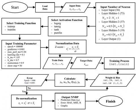
This study used Matlab’s Graphical User Interface (GUI) in performing data training, testing, and prediction when simulating the ANN-BP algorithm with three hidden layers. Inputs, processes, and data outputs were displayed in a single GUI. The GUI output displays prediction result data, actual data approach graph and forecasting data, as well as accuracy rate parameters [15, 49].
$M S E=\frac{\sum_{i=1}^n\left(A_i-F_i\right)^2}{n}$ (6)
$R M S E=\left(\frac{\sum_{i=1}^n\left(A_i-F_i\right)^2}{n}\right)^{\frac{1}{2}}$ (7)
Then, the climate classification used the Schmidt-Ferguson criteria. The basis of the Schmidt-Ferguson climate classification (Q) is the amount of precipitation that falls each month so that the average wet, humid, and dry month all recorded [50]. The categories of months were categorized as follows: wet months (WM) with rainfall greater than 100mm/month, humid months (HM) with rainfall of 60-100mm/month, and dry months (DM) with a rainfall of approximately 60mm/month. There are seven climate classifications as seen on Table 3.
Table 3. The type of climate based on Q value [51, 52]
|
Formula |
Q Value |
Climate |
Type of Climate |
Information |
|
$Q=\frac{D M}{W M}$
DM: dry month WM: wet month |
Q<0.14 |
A |
Very wet |
Tropical rainforest |
|
0.14≤Q<0.33 |
B |
Wet |
Tropical rainforest |
|
|
0.33≤Q<0.66 |
C |
Rather wet |
Forest |
|
|
0.66≤Q<1.00 |
D |
Medium |
Season forest |
|
|
1.00≤Q<1.67 |
E |
Rather dry |
Savanna forest |
|
|
1.67≤Q<3.00 |
F |
Dry |
Savanna forest |
|
|
3.00≤Q<7.00 |
G |
Very dry |
Grassland |
|
|
Q≥7.00 |
H |
Extreme |
Grassland |
3.1 ANN-BP architecture with three hidden layers
From Figure 1 and Eq. (1), more than 1 hidden layer, e.g. three hidden layers, can be developed. Figure 3 shows a piece or section of ANN-BP architecture with three hidden layers.
Figure 3. ANN Backpropagation architecture section with three hidden layers
Figure 3 indicates the addition of a hidden layer along with a matrix of the weight of each layer according to Table 4 below.
Table 4. ANN-BP architecture variables with 3 hidden layers
|
Layer |
Layer Variables |
Weight Variables |
|
Layer Input |
$x_1, x_2, \ldots, x_i, \ldots, x_n$ |
- |
|
Layer Hidd-1 |
$z_1, z_2, \ldots, z_j, \ldots, z_p$ |
$v_{11}, v_{1 j}, \ldots, v_{i j}, \ldots, v_{n p}$ |
|
Layer Hidd-2 |
$z a_1, z a_2, \ldots, z a_q, \ldots, z a_s$ |
$w_{11}, w_{1 s}, \ldots, w_{j q}, \ldots, w_{p s}$ |
|
Layer Hidd-3 |
$z b_1, z b_2, \ldots, z b_r, \ldots, z b_t$ |
$w a_{11}, w a_{1 r}, \ldots, w a_{g r}, \ldots, w a_{s t}$ |
|
Layer Output |
$y_1, y_2, \ldots, y_k, \ldots, y_m$ |
$w b_{11}, w b_{1 k}, \ldots, w b_{r k}, \ldots, w b_{t m}$ |
Based on Table 4, a formula can be formed for data prediction with three hidden layers. Referring to the number of neurons that have been determined in each layer, namely 36-73-37-19-1, the following mathematical model of rainfall prediction is obtained.
$y_k=f\left(w b_{0 k}+\sum_{r=1}^t w b_{r k} \cdot f\left(w a_{0 r}+\sum_{q=1}^s w a_{q r} \cdot f\left(w_{0 q}+\sum_{j=1}^p w_{j q} \cdot f\left(v_{0 j}+\sum_{i=1}^n v_{i j} \cdot x_i\right)\right)\right)\right)$ (8)
$y_k=f_o\left(w b_{0 k}+\sum_{r=1}^{19} w b_{r k} \cdot f_{H 3}\left(w a_{0 r}+\sum_{q=1}^{37} w a_{q r} \cdot f_{H 2}\left(w_{0 q}+\sum_{j=1}^{73} w_{j q} \cdot f_{H 1}\left(v_{0 j}+\sum_{i=1}^{36} v_{i j} \cdot x_i\right)\right)\right)\right)$ (9)
The activation function $f_o(.)$ is an activation function on the output layer, $f_{H 1}(.)$ is an activation function on the first hidden layer, $f_{H 2}(.)$ is an activation function on the second hidden layer, and $f_{H 3}(.)$ is an activation function on the third hidden layer. These activation functions include identity functions, binary sigmoids, bipolar sigmoids, and hyperbolic tangents combined on each hidden layer and output layer along with training functions (trainrp and trainlm) during the data training and testing process. The results of training and testing data were tabulated to analyze the network architecture with the highest level of accuracy with the lowest error. The procedure of training data and testing data is presented in Figure 4.
Figure 4. Data prediction procedure with three hidden layers
Figure 4 shows that all input data are trained using a three-layer hidden architecture. All input data, a total of 36 data, need to be trained after normalization by Z-score technique, and then process the input data in the first hidden layer of 73 neurons according to the determined activation function and training function (see Table 5). The output of the first hidden layer is passed to the second hidden layer with 37 neurons and on to the third hidden layer with 19 neurons. Continue training with data from input layer to output layer until target/error 0.001 is reached.
3.2 Results of training, testing, and prediction data
After the computational scripts and GUI ANN Backpropagation were completed, the further process of training and testing data using architecture 36-73-37-19-1 was performed. On this occasion, the authors applied the concept of conventional combinations for activation functions. The results of the training and testing data process are shown in Table 5.
Table 5 shows that the best architecture in the data training process is obtained by a combination of the activation function "logsig-logsig-logsig-purelin" in the classification of "variations type-1" with an epoch of 7, MSE of 0.00090, and RMSE of 0.03011, and in the data testing process with an epoch of 5, MSE of 0.003758, and RMSE of 0.0613. The results of training and testing using the same type of non-variation or training function in each layer obtained poor results with elevated MSE and RMSE values and a high epoch. The results of the tansig and tanh function training also provided a high number of epochs up to more than 50,000 iterations when using the trainrp function. Meanwhile, the training process with the trainlm function took a very long time (more than 1 hour) and when the process was stopped, it only obtained an average goal of 0.16-0.54 > 0.001. These results show that the combination of the tansig and tanh activation functions with the trainrp function is not recommended for the data prediction process. In addition, the results of variations type-2 with the combination of each layer and different activation functions would provide invalid training results with the lowest MSE value of 171,067 (tansig-tanh-logsig-purelin function) and RMSE value higher than 10. The graph of the actual data approach and the target of training and testing data results are presented in Figure 5 and Figure 6.
Table 5. Result of training and testing data
|
Combination activation |
Training function |
Training |
Testing |
||||
|
Epoch |
MSE |
RMSE |
Epoch |
MSE |
RMSE |
||
|
Variations |
|||||||
|
P-P-P-P |
trainrp |
203 |
1904.82 |
43.6443 |
3444 |
2.8859 |
1.6988 |
|
trainlm |
5 |
1904.82 |
43.6443 |
3 |
0.9685 |
0.9841 |
|
|
L-L-L-L |
trainrp |
1493 |
1980.65 |
44.5045 |
235 |
1544.95 |
39.3058 |
|
trainlm |
322 |
1950.82 [0.54]* |
44.1681 |
285 |
1382.28 [0.45]* |
37.179 |
|
|
T-T-T-T |
trainrp |
53,873 |
1725.50 |
41.5392 |
27,564 |
768.258 |
27.7175 |
|
trainlm |
136 |
3036.94 [0.25]* |
55.1085 |
162 |
2513.55 [0.16]* |
50.1353 |
|
|
Th-Th-Th-Th |
trainrp |
51,010 |
1845.51 |
42.9593 |
23,923 |
462.933 |
21.5159 |
|
trainlm |
122 |
912.498 [0.25] |
30.2076 |
116 |
462.93 [0.16] |
21.5158 |
|
|
Variations Type-1 |
|||||||
|
L-L-L-P |
trainrp |
59 |
3.49472 |
1.86942 |
30 |
2.35792 |
1.53555 |
|
trainlm |
7 |
0.00090 |
0.03011 |
5 |
0.003758 |
0.0613 |
|
|
T-T-T-P |
trainrp |
89 |
1479.55 |
38.4649 |
33 |
389.973 |
19.7477 |
|
trainlm |
6 |
1772.78 |
42.1044 |
3 |
2243.02 |
47.3605 |
|
|
Th-Th-Th-P |
trainrp |
115 |
3.61946 |
1.90249 |
36 |
2.5385 |
1.5932 |
|
trainlm |
7 |
0.02037 |
0.14274 |
3 |
0.3428 |
0.5855 |
|
|
Variations Type-2 |
|||||||
|
Th-L-T-P |
trainrp |
76 |
445.674 |
21.111 |
30 |
233.839 |
15.2918 |
|
trainlm |
6 |
440.493 |
20.987 |
4 |
742.533 |
27.2495 |
|
|
Th-T-L-P |
trainrp |
72 |
190.224 |
13.792 |
30 |
39.061 |
6.2498 |
|
trainlm |
7 |
484.42 |
22.009 |
4 |
222.234 |
14.9075 |
|
|
L-Th-T-P |
trainrp |
76 |
238.378 |
15.439 |
31 |
396.344 |
19.9084 |
|
trainlm |
15 |
639.337 |
25.285 |
4 |
480.47 |
21.9196 |
|
|
L-T-Th-P |
trainrp |
92 |
252.141 |
15.879 |
29 |
450.152 |
21.2168 |
|
trainlm |
7 |
725.288 |
26.931 |
3 |
452.364 |
21.2688 |
|
|
T-Th-L-P |
trainrp |
110 |
171.067 |
13.079 |
37 |
26.767 |
5.17369 |
|
trainlm |
7 |
383.614 |
19.586 |
3 |
708.789 |
26.6231 |
|
|
T-L-Th-P |
trainrp |
64 |
160.966 |
12.687 |
25 |
52.4609 |
7.24299 |
|
trainlm |
6 |
774.656 |
27.8326 |
3 |
511.856 |
22.6242 |
|
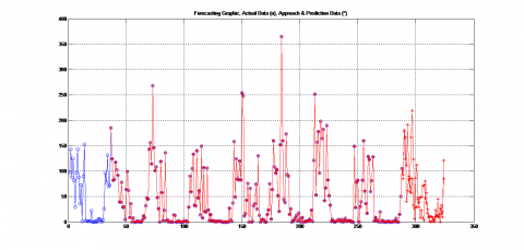
Figure 5. Approach of actual data (o-blue) and target data or prediction (*-red) in the training process
Figure 6. Approach of actual data (o-blue) and target data or prediction (*-red) in the testing process
Figure 5 shows that the input data or actual data $\left(x_1, x_2, x_3, \ldots, x_{288}\right)$, approaches the target data $\left(x_{37}, x_{38}, x_{39}, \ldots, x_{324}\right)$ are impeccable, where data $x_{289}, x_{290}, x_{291}, \ldots, x_{324}$ are prediction data, with MSE of 0.00090 and RMSE of 0.03011. While, Figure 6 shows that the actual data $\left(x_1, x_2, x_3, \ldots, x_{72}\right)$ are also close to the target dat $\left(x_{37}, x_{38}, x_{39}, \ldots, x_{108}\right)$ perfectly, where data $x_{73}, x_{74}, x_{75}, \ldots, x_{108}$ are prediction data, with MSE of 0.003758 and RMSE of 0.0613. Based on the results of training and testing data, the best performance was obtained by using the trainlm function. This result is similar with the research result of Almaliki et al. [53] who predicted tractor performance under different field conditions with an R2 value of 0.989 and MSE of 0.001327. The prediction of specific wear rate for LM25/ZrO2 composites using ANN-BP with Levenberg–Marquardt function also provided good performance with an accuracy rate of up to 99% [54]. This result is also similar with the research result of Sun and Huang [48] who reported that the use of a learning rate of 0.1 provided high accuracy during the training and data testing process. This is also in line with the study of Bai et al. [55] who made predictions of air pollutants with the trainlm function and obtained a coefficient correlation value of 0.926. Furthermore, the logsig activation function provided the best model to determine input data patterns. Because the binary sigmoid activation function (logsig) is very suitable for use in forecasting that uses fluctuating data. The data output is not zero-centered because the logsig function is a continuous function with the output target being at intervals [0, 1]. It is clear that the data used in the study is rainfall data that has high fluctuations. Finally, an important finding in the study was the use of ANN Backpropagation architecture with three hidden layers had an accuracy rate of up to 99% although it required a longer training time than the architecture with one or two hidden layers. Furthermore, the network architecture was used to make short-term predictions, such as data prediction in 2022 using data in 2012-2021. The prediction results were presented in Figure 7.
Figure 7. Results of predicted rainfall data in 2022
The prediction result (Figure 7) was obtained with an epoch of 11, MSE of 0.0011, RMSE of 0.0328, and R2 of 0.9999. Figure 7 illustrates that the highest rainfall intensity in the area around Lombok International Airport (BIL) in 2022 will be in November (566.28 mm), while the lowest would be in May (21.81 mm). Based on the climate classification by Schmidt-Ferguson criteria, there are 9 wet months with high rainfall intensity, including January, February, March, April, July, September, October, November, and December; one humid month, namely June; and two dry months, namely May and August. It can be reported that this region belongs to the type B climate (Q-value = 0.222) or the "wet" climate. This result is different from that of the previous years, except the 2016 results with the same Q and category values. Table 6 shows that in the region around BIL stations there is a different intensity of rain each year, but it is not very significant. The change in the number of "wet" months since the last four years has increased.
Table 6. Climate categories each year
|
Years |
Number of Month |
Q |
Type of Climate |
||
|
Wet |
Dry |
Humid |
|||
|
2012 |
7 |
5 |
0 |
0.714 |
D-Medium |
|
2013 |
8 |
4 |
0 |
0.500 |
C-Rather wet |
|
2014 |
6 |
6 |
0 |
1.000 |
E-Rather dry |
|
2015 |
5 |
7 |
0 |
1.400 |
E-Rather dry |
|
2016 |
9 |
2 |
1 |
0.222 |
B-Wet |
|
2017 |
6 |
6 |
0 |
1.000 |
E-Rather dry |
|
2018 |
5 |
7 |
0 |
1.400 |
E-Rather dry |
|
2019 |
5 |
7 |
0 |
1.400 |
E-Rather dry |
|
2020 |
7 |
4 |
1 |
0.571 |
C-Rather wet |
|
2021 |
7 |
4 |
1 |
0.571 |
C-Rather wet |
|
2022 |
9 |
2 |
1 |
0.222 |
B-Wet |
Climate change can be indicated by an increasing or decreasing monthly rainfall intensity, which should be an important concern, especially for governments in taking strategic measures to prevent negative impacts. Various policies are essential to be observed in order to reduce risks of errors at the implementation stage. Especially for policies on agriculture, the government needs to draw up planting pattern plans and convey climate change information to farmers to avoid crop failure.
The output of the artificial neural network provides information that there will be climate change in 2022, where the intensity of rainfall is higher with 9 "wet" months, 1 "dry" month, and 2 "humid" months. The Q-value of 0.222 based on the Schmidt-Ferguson criteria should be an important concern, especially as the government needs to draw up planting pattern plans and convey climate change information to farmers to avoid crop failure. This prediction was obtained from the results of ANN Backpropagation architecture simulation with three hidden layers. The results of training and data testing showed that the 36-73-37-19-1 architecture with variations in activation functions, namely logsig-logsig-logsig-purelin, has the highest level of accuracy compared to other function variations. The trainlm function provides better performance than trainrp. Although the trainlm function takes longer training time, the number of iterations, MSE, and RMSE are relatively lower than that of the trainrp. This architecture needs to be re-tested in other case studies, such as studies on temperature data, air humidity, wind speed, and the length of sunlight, to measure the accuracy level of network that has been created in recognizing data patterns that have different trends.
[1] Hendrix, C.S., Salehyan, I. (2012). Climate change, rainfall, and social conflict in Africa. Journal of Peace Research, 49(1): 35-50. https://doi.org/10.1177/0022343311426165
[2] Dos Santos, S.M., de Farias, M.M.M. (2017). Potential for rainwater harvesting in a dry climate: Assessments in a semiarid region in northeast Brazil. Journal of Cleaner Production, 164: 1007-1015. https://doi.org/10.1016/j.jclepro.2017.06.251
[3] Bello, A., Mamman, M. (2018). Monthly rainfall prediction using artificial neural network: A case study of Kano, Nigeria. Environmental and Earth Sciences Research Journal, 5(2): 37-41. https://doi.org/10.18280/eesrj.050201
[4] Pramita, D., Nusantara, T., Negara, H.R.P. (2020). Analysis of accuracy parameters of ANN backpropagation algorithm through training and testing of hydro-climatology data based on GUI MATLAB. IOP Conference Series: Earth and Environmental Science, 413(1). https://doi.org/10.1088/1755-1315/413/1/012008
[5] Zhang, Q., Li, Z., Zhu, L., Zhang, F., Sekerinski, E., Han, J.C., Zhou, Y. (2021). Real-time prediction of river chloride concentration using ensemble learning. Environmental Pollution, 291. https://doi.org/10.1016/j.envpol.2021.118116
[6] Shu, X., Ding, W., Peng, Y., Wang, Z., Wu, J., Li, M. (2021). Monthly streamflow forecasting using convolutional neural network. Water Resources Management, 35(15): 5089-5104. https://doi.org/10.1007/s11269-021-02961-w
[7] Abbot, J., Marohasy, J. (2017a). Application of artificial neural networks to forecasting monthly rainfall one year in advance for locations within the murray darling basin, Australia. International Journal of Sustainable Development and Planning, 12(8): 1282-1298. https://doi.org/10.2495/SDP-V12-N8-1282-1298
[8] Khan, R.S., Bhuiyan, M.A.E. (2021). Artificial intelligence-based techniques for rainfall estimation integrating multisource precipitation datasets. Atmosphere, 12(10): 1-14. https://doi.org/10.3390/atmos12101239
[9] Diagi, B. (2018). Analysis of rainfall trend and variability in Ebonyi state, South Eastern Nigeria. Environmental and Earth Sciences Research Journal, 5(3): 53-57. https://doi.org/10.18280/eesrj.050301
[10] Abbot, J., Marohasy, J. (2017). Forecasting extreme monthly rainfall events in regions of Queensland, Australia using artificial neural networks. International Journal of Sustainable Development and Planning, 12(7): 1117-1131. https://doi.org/10.2495/SDP-V12-N7-1117-1131
[11] Traore, S., Wang, Y.M., Kerh, T. (2010). Artificial neural network for modeling reference evapotranspiration complex process in Sudano-Sahelian zone. Agricultural Water Management, 97(5): 707-714. https://doi.org/10.1016/j.agwat.2010.01.002
[12] Mislan, H., Hardwinarto, S., Sumaryono, M.A., Aipassa, M. (2015). Rainfall monthly prediction based on artificial neural network: A case study in Tenggarong Station, East Kalimantan - Indonesia. Procedia Computer Science, 59: 142-151. https://doi.org/10.1016/j.procs.2015.07.528
[13] Russell, S., Norvig, P. (2010). Artificial Intelligence a Modern Approach Third Edition. In Pearson. https://doi.org/10.1017/S0269888900007724
[14] Lau, M.M., Lim, K.H. (2019). Review of adaptive activation function in deep neural network. 2018 IEEE EMBS Conference on Biomedical Engineering and Sciences, IECBES 2018 - Proceedings, 686-690. https://doi.org/10.1109/IECBES.2018.08626714
[15] Sinharoy, A., Baskaran, D., Pakshirajan, K. (2020). Process integration and artificial neural network modeling of biological sulfate reduction using a carbon monoxide fed gas lift bioreactor. Chemical Engineering Journal, p. 391. https://doi.org/10.1016/j.cej.2019.123518
[16] Kumar, D.A., Murugan, S. (2018). Performance analysis of NARX neural network backpropagation algorithm by various training functions for time series data. International Journal of Data Science, 3(4): 308. https://doi.org/10.1504/ijds.2018.096265
[17] Supriyanto, E.E., Septyanun, N., Harun, R.R., Apriansyah, D., Saputra, E. (2021). ANN Back Propagation in forecasting and policy analysis on family planning programs: A case study in NTB Province. Journal of Physics: Conference Series, 1882(1). https://doi.org/10.1088/1742-6596/1882/1/012036
[18] Lahmiri, S. (2012). An EGARCH-BPNN system for estimating and predicting stock market volatility in Morocco and Saudi Arabia: The effect of trading volume. Management Science Letters, 2(4): 1317-1324. https://doi.org/10.5267/j.msl.2012.02.007
[19] Abdelkader, E.M., Al-Sakkaf, A., Ahmed, R. (2020). A comprehensive comparative analysis of machine learning models for predicting heating and cooling loads. Decision Science Letters, 9(3): 409-420. https://doi.org/10.5267/j.dsl.2020.3.004.
[20] Mohandes, S.R., Zhang, X., Mahdiyar, A. (2019). A comprehensive review on the application of artificial neural networks in building energy analysis. Neurocomputing, 340: 55-75. https://doi.org/10.1016/j.neucom.2019.02.040
[21] Pandey, S., Hindoliya, D.A., Mod, R. (2012). Artificial neural networks for predicting indoor temperature using roof passive cooling techniques in buildings in different climatic conditions. Applied Soft Computing Journal, 12(3): 1214-1226. https://doi.org/10.1016/j.asoc.2011.10.011
[22] Lahmiri, S. (2011). A comparative study of Backpropagation algorithms in financial prediction. International Journal of Computer Science, Engineering and Applications, 1(4): 15-21. https://doi.org/10.5121/ijcsea.2011.1402
[23] Kumar, D.A., Murugan, S. (2014). Performance analysis of MLPFF neural network back propagation training algorithms for time series data. Proceedings - 2014 World Congress on Computing and Communication Technologies, WCCCT 2014, 114-119. https://doi.org/10.1109/WCCCT.2014.47
[24] Sharawat, S. (2012). Software maintainability prediction using neural networks. Ijera, 2(2): 750-755. http://www.ijera.com/pages/v2no2.html
[25] Khong, L.M.D., Gale, T.J., Jiang, D., Olivier, J.C., Ortiz-Catalan, M. (2013). Multi-layer perceptron training algorithms for pattern recognition of myoelectric signals. BMEiCON 2013 - 6th Biomedical Engineering International Conference. https://doi.org/10.1109/BMEiCon.2013.6687665
[26] Samani, A. (2018). Combined cycle power plant with indirect dry cooling tower forecasting using artificial neural network. Decision Science Letters, 7(2): 131-142. https://doi.org/10.5267/j.dsl.2017.6.004
[27] Jigyasu, R., Mathew, L., Sharma, A. (2019). Multiple faults diagnosis of induction motor using artificial neural network. Communications in Computer and Information Science, 955: 701-710. https://doi.org/10.1007/978-981-13-3140-4_63
[28] Elkharbotly, M.R., Seddik, M., Khalifa, A. (2022). Toward sustainable water: Prediction of non-revenue water via Artificial Neural Network and Multiple Linear Regression modelling approach in Egypt. Ain Shams Engineering Journal, 13(5): 1-16. https://doi.org/https://doi.org/10.1016/j.asej.2021.101673
[29] Kuruvilla, J., Gunavathi, K. (2014). Lung cancer classification using neural networks for CT images. Computer Methods and Programs in Biomedicine, 113(1): 202-209. https://doi.org/10.1016/j.cmpb.2013.10.011
[30] Yang, J., Du, L., Shi, S., Gong, W., Sun, J., Chen, B. (2019). Potential of fluorescence index derived from the slope characteristics of laser-induced chlorophyll fluorescence spectrum for rice leaf nitrogen concentration estimation. Applied Sciences (Switzerland), 9(5): 1-12. https://doi.org/10.3390/app9050916
[31] Yuwono, K.A., Safitri, I., Tritoasmoro, I.I. (2019). Artificial Neural Networks Android-Based Interface Facial Recognition Systems. 2019 2nd International Seminar on Research of Information Technology and Intelligent Systems, ISRITI 2019: 248-252. https://doi.org/10.1109/ISRITI48646.2019.9034569
[32] Otache, M.Y., Musa, J.J., Kuti, I.A., Mohammed, M., Pam, L.E. (2021). Effects of model structural complexity and data pre-processing on Artificial Neural Network (ANN) forecast performance for hydrological process modelling. Open Journal of Modern Hydrology, 11(1): 1-18. https://doi.org/10.4236/ojmh.2021.111001
[33] Pramita, D., Nusantara, T. (2021). Forecasting using back propagation with 2-layers hidden. Journal of Physics: Conference Series. https://doi.org/10.1088/1742-6596/1845/1/012030
[34] Asgari, H., Chen, X., Menhaj, M.B., Sainudiin, R. (2013). Artificial neural network-based system identification for a single-shaft gas turbine. Journal of Engineering for Gas Turbines and Power, 135(9): 1-7. https://doi.org/10.1115/1.4024735
[35] kmi, A.M. (2013). Intelligent irrigation water requirement system based on artificial neural networks and profit optimization for planting time decision making of crops in Lombok Island. Journal of Theoretical and Applied Information Technology, 58(3): 657-671. http://www.jatit.org/volumes/Vol58No3/22Vol58No3.pdf.
[36] Fausett, L. (1994). Fundamentals of Neural Network. Prentice Hall.
[37] Tepedelenlioglu, N., Rezgui, A. (1989). The effect of the activation function of the back propagation algorithm. IEEE 1989 International Conference on Systems Engineering, pp. 139-145. https://doi.org/10.1109/ICSYSE.1989.48639
[38] Fletcher, G.P. (1996). Adaptive internal activation functions and their effect on learning in feed forward networks. Neural Processing Letters, 4(1): 29-38. https://doi.org/10.1007/BF00454843
[39] Singh, B.K., Verma, K., Thoke, A.S. (2015). Adaptive gradient descent backpropagation for classification of breast tumors in ultrasound imaging. Procedia Computer Science, 46: 1601-1609. https://doi.org/10.1016/j.procs.2015.02.091
[40] Tarigan, J., Diedan, R., Suryana, Y. (2017). Plate recognition using backpropagation neural network and genetic algorithm. Procedia Computer Science, 116: 365-372. https://doi.org/10.1016/j.procs.2017.10.068
[41] Paeedeh, N., Ghiasi-Shirazi, K. (2021). Improving the backpropagation algorithm with consequentialism weight updates over mini-batches. Neurocomputing, 461: 86-98. https://doi.org/10.1016/j.neucom.2021.07.010
[42] Mustafidah, H., Hartati, S., Wardoyo, R., Harjoko, A. (2014). Selection of most appropriate backpropagation training algorithm in data pattern recognition. International Journal of Computer Trends and Technology (IJCTT), 14(2): 92-95. https://doi.org/https://doi.org/10.14445/22312803/IJCTT-V14P120
[43] Utomo, D. (2017). Stock price prediction using back propagation neural network based on gradient descent with momentum and adaptive learning rate. Journal of Internet Banking and Commerce, 22(3): 16.
[44] Baum, E.B., Haussler, D. (1989). What size net gives valid generalization? Neural Computation, 1(1): 151-160. https://doi.org/10.1162/neco.1989.1.1.151
[45] Hecht-Nielsen, R. (1987). Kolmogorov’s mapping neural network existence theorem. Proceedings of the International Conference on Neural Networks, pp. 11-14. https://cir.nii.ac.jp/crid/1571698599617740928.
[46] Park, H. (2011). Study for application of artificial neural networks in geotechnical problems. In Artificial Neural Networks - Application, pp. 303-336. https://doi.org/10.5772/15011
[47] Datt, G., Bhatt, A.K., Saxena, A. (2021). An investigation of artificial neural network based prediction systems in rain forecasting. International Journal on Recent and Innovation Trends in Computing and Communication, 3(8): 5338-5349. https://doi.org/https://doi.org/10.17762/ijritcc.v3i8.4841
[48] Sun, W., Huang, C. (2020). A carbon price prediction model based on secondary decomposition algorithm and optimized back propagation neural network. Journal of Cleaner Production, p. 243. https://doi.org/10.1016/j.jclepro.2019.118671.
[49] Nastos, P.T., Moustris, K.P., Larissi, I.K., Paliatsos, A.G. (2013). Rain intensity forecast using Artificial Neural Networks in Athens, Greece. Atmospheric Research, 119: 153-160. https://doi.org/10.1016/j.atmosres.2011.07.020
[50] Wijayanti, R., Saleh, E., Hanum, H., Aprianti, N. (2020). Climate change analysis (monthly rainfall) on Palembang Duku production (Lansium domesticum Corr). Sriwijaya Journal of Environment, 5(2): 120-126. https://doi.org/10.22135/sje.2020.5.2.120-126
[51] Saiya, H.G., Hiariej, A., Pesik, A., Kaya, E., Hehanussa, M.L., Puturuhu, F. (2020). Dispersion of tongka langit banana in buru and seram, maluku province, indonesia, based on topographic and climate factors. Biodiversitas, 21(5): 2035-2046. https://doi.org/10.13057/biodiv/d210529
[52] Irfan, M. (2006). The determination of Palembang climate type by using Schmidt-Ferguson method. Joint International Conference on “Sustainable Energy and Environment, 1(1): 1-2. https://citeseerx.ist.psu.edu/viewdoc/download?doi=10.1.1.385.6817
[53] Almaliki, S., Alimardani, R., Omid, M. (2016). Artificial neural network based modeling of tractor performance at different field conditions. Agricultural Engineering International: CIGR Journal, 18(4): 262-274. https://cigrjournal.org/index.php/Ejounral/article/view/3880.
[54] Kannaiyan, M., Karthikeyan, G., Raghuvaran, J.G.T. (2020). Prediction of specific wear rate for LM25/ZrO2 composites using Levenberg-Marquardt backpropagation algorithm. Journal of Materials Research and Technology, 9(1): 530-538. https://doi.org/10.1016/j.jmrt.2019.10.082
[55] Bai, Y., Li, Y., Wang, X., Xie, J., Li, C. (2016). Air pollutants concentrations forecasting using back propagation neural network based on wavelet decomposition with meteorological conditions. Atmospheric Pollution Research, 7(3): 557-566. https://doi.org/10.1016/j.apr.2016.01.004