Simulation Study of Integrated Solar Combined Cycle Systems: Medium Scale Plant in Irbid City

The system is composed of the solar system Concentrating solar power (CSP) and vapor power cycle (Rankin cycle). The power cycle is driven by the heat, which is produced by the solar system as shown in Figure 1. The components of the steam cycle are steam generators (Overheater, Evaporator and Economizer).

Presentation of the CSP –thermal power plant used CSP technologies-The Parabolic Trough Solar Collector (PTC) type can be used to generate electricity during the sunny day hours throughout the year. This technology has the ability to store energy as a result of its configuration, which consists of a mirror that concentrates the sun's light energy and converts it to heat. Then, heat can be used to generate steam to produce electrical energy through a steam turbine. The PTC contains a receiver tube (RT) and a parabolic-cylindrical mirror (parallel rows of long, semi-cylindricals) which circles around the RT to increase the concentration of radiation. The sun's radiation is concentrated on a longitudinal RT which is arranged along the installation. A Heat Transfer Fluid (HTF) – a type of THERMINOL VP-1 - circulates inside the RT, which is used to capture and transport the absorbed heat; the thermal liquid temperature can reach up to 300℃. The THERMINOL VP-1 used as a thermal liquid circulates inside the solar field (PTC) in order to overcome the mechanical constraints in the case of the immediate evaporation of water in the solar collector [32-34]. Moreover, the heat is transmitted to the cold water and transferred it to the steam (at efficiency in the range of 14- 21%), which is used to operate the steam turbine. This system is made up of molten salt storage that can be kept during non-sunday hours.

Three stages of the steam turbine (low pressure LP, intermediate pressure IP, and high pressure HP), collector field (PTC), preheater, degasser, sub-cooler, condenser, and pump. The aim of the collector field is to generate electricity from the thermal system. The system consists of the PTC connected to the steam turbine - Rankine cycle through a set of heat exchangers. The average temperature of the thermal fluid increases according to the weather during the day and year (8760 h). The heat transfer fluid (thermal fluid) is pumped to the steam generator (economizer, evaporator, and superheater) at a constant flow rate. The HTF exchanges its heat with water (working fluid) through a heat exchanger where the HFT flows in the opposite direction of water flow. As shown in Figure 1, the HFT passes through the superheater to raise the temperature of the steam generated in the evaporator, then through the evaporator to release its heat and convert the warm water phase to a vapor. The HFT exits from the last stage of the steam generator and releases the last portion of its heat to heat the water inside the economizer, which leads to an increase in the water temperature. Then the HFT returns to the solar field to absorb the solar energy again. In the power cycle, the superheated steam completes its cycle by passing through three stages of the steam turbine.

1.png

Figure 1. Schematic diagram of the thermal power cycle - solar field system

The steam turbine is divided into three stages: LP, IP, and HP, which all communicate with the preheaters (feed-water heaters). A portion of the steam (approximately 0.13% of steam) is withdrawn during the expansion and is used to heat the feed water in order to increase the efficiency of the cycle. The remaining saturation steam exits from the LP stage with low enthalpy and enters the condenser. In the condenser, the steam releases its heat and condenses. Two pumps are used to increase the pressure as required by the steam generator and the water passes through a degreaser in order to remove the melted gases before entering the steam generator.

The advanced model requires the site's geographical position and the typical metrological year (TMY) data that generates hourly metrological data, which includes wind speed and ambient temperature. The Global Land Data Assimilation System (GLDAS-version 1) provides estimates for all of the variables studied. The Global Data Assimilation System is a system of operational atmospheric analysis that combines a model of the global climate–a numerical depiction of the energy fluxes and physical processes occurring in the earth's atmosphere, land surface, and oceans–with a diverse set of satellite-derived analyses and observations. In order to run the simulation for one year and to predict the system, the TMY of Irbid is used at the GMT+2 time zone, latitude 32.5514450 N, and longitude 35.851479.

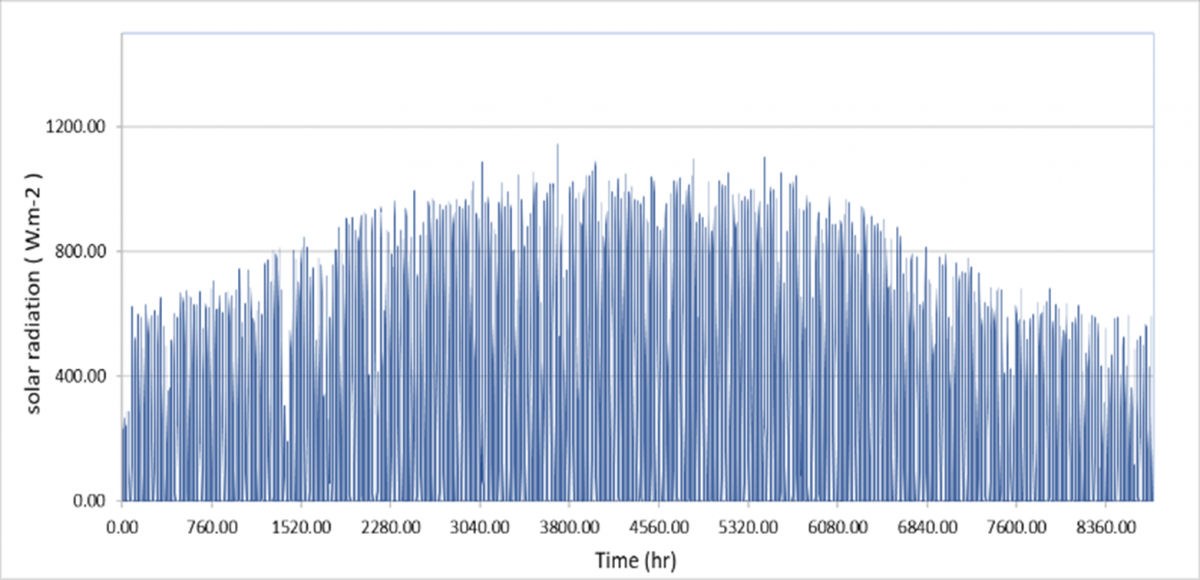
4.1 Solar radiation, dry bulb temp and wind speed

The total horizontal radiation (direct and diffuse radiation on the horizontal surface) in Irbid city is evaluated as shown in Figure 3a. During the months of May and June, the maximum radiation obtained is approximately 1145 W/m².

It is noted that Irbid city has high irradiation, especially during June, while the lowest irradiation is received during December. The reason for that is due to the location of Irbid, the scarcity of clouds, and the low humidity, which positively affects the arrival of direct horizontal solar radiation to the earth.

3a.png

(a)

3b.png

(b)

3c.png

(c)

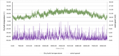
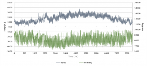
Figure 3. (a). Solar radiation in Irbid city; (b). Wind speed and dry bulb temp over year in Irbid; (c). A variations in temperature and annual average humidity in Irbid

Figure 3c shows ambient temperature over the year. The period between May and Jun is characterized by maximum ambient temperature and speed wind (see Figure 3b). Wind speed seems to have a significant impact on the energy production of a solar module. Indeed, the heat transfer coefficient may be defined as a function of total irradiance, ambient temperature, and wind speed. This coefficient particularly follows a linear law instead of the constant value usually taken into consideration by PV software such as PVsyst.

The maximum ambient temperature and speed of wind registered were 37°C and 14.772 m/s., respectively. That is related to the total sunshine hours during the summer, which are longer than those during the winter. In addition, the sun's steadiness in the northern hemisphere, as the rays of the sun are almost perpendicular during the summer to the surface of the earth, makes the earth absorb most of the radiation energy and only a small portion is reflected from it, unlike in winter where the rays are highly inclined, which leads to reflecting the radiation without absorption.

The annual average humidity over the year. For the variation of the average annual moisture content in Irbid, it has been observed that it is lower during summer (range of 0.48-0.63) than winter (range of 0.63-0.82).

4.2 Thermal performance evaluation of the system

The curve illustrated in Figure 4a shows that at the beginning of the heating on January 1, at t=0 (24:00), the outlet temperature of the coolant is equal to the temperature of the injected fluid. After the sun rises, this temperature increases with the solar radiation concentrated on the concentrator opening. The temperature reaches 240 °C between 7:00 h (am) and 4:00 h (pm). During the same time period, the inlet temperature reaches 217°C and rises to a maximum of 290.92°C at 11:00 h (am). During the afternoon, both inlet and outlet temperatures after 5:00 h (pm) continue to decrease until they reach zero.

4a.png

(a)

4b.png

(b)

Figure 4. A Variation of PTC fluid inlet and outlet temperature (a) during the Day of January 1, (b) during the Day of August 1

Figure 4b shows the same behavior of the HTF temperature on January 1, with an increased peak temperature of the inlet and outlet of the HTF during the period of 8:00 h (am) to 4:00 h (pm). The number of sunny hours on August 1 is greater than on January 1, resulting in an increase in energy yield. Also, the irradiation is more perpendicular, which is reflected in the increment in the coolant temperature. The inlet and outlet temperatures of the HTF reached the maximum values of 392°C and 361°C, respectively. An increment is noted before 8:00 h (am) and a decrement after 4:00 h (pm) as a result of the radiation incident angle.

4.3 Steam generator temperatures and Transferred power

The curves illustrated in Figure 5a and b show that the temperatures of the steam generator fluid on the cold and hot and cold sides increase to a peak at around 14 hr at the inlet of the steam generator. This period corresponds to maximum sun radiation. Regarding the cold side (outlet), it should be noted that the temperature will rise at each stage, reaching a maximum of 327°C at 13:00 h. After 13:00 h, the exit temperatures on each side will decrease when the sun irradiation declines until 18:00 h or they will be zero.

The temperature profiles of the steam generator fluid (working fluid) between January 1 and August 1 were obtained as shown in Figures 5a and 5b. The behavior of the temperature of the working fluid reflects the high thermal efficiency of the steam generator, with slight variance between the generator components (superheater, evaporator, and the economizer). As shown in Figure 6a and b. In this simulation, by the comparison of the inlet and outlet temperature of the coolant and working fluid, it is clearly the heat transfer between two fluids very high that will increase the system gain. This can be considered by efficiency, which can be expressed as Qout/Qin, Qout is the heat absorbed by cold water, and Qin is the heat absorbed by the working fluid.

5a.png

(a)

5b.png

(b)

Figure 5. Variation of steam generator temperatures of the fluid on the hot and cold sides (a) during the Day of January, (b) during the Day of August 1

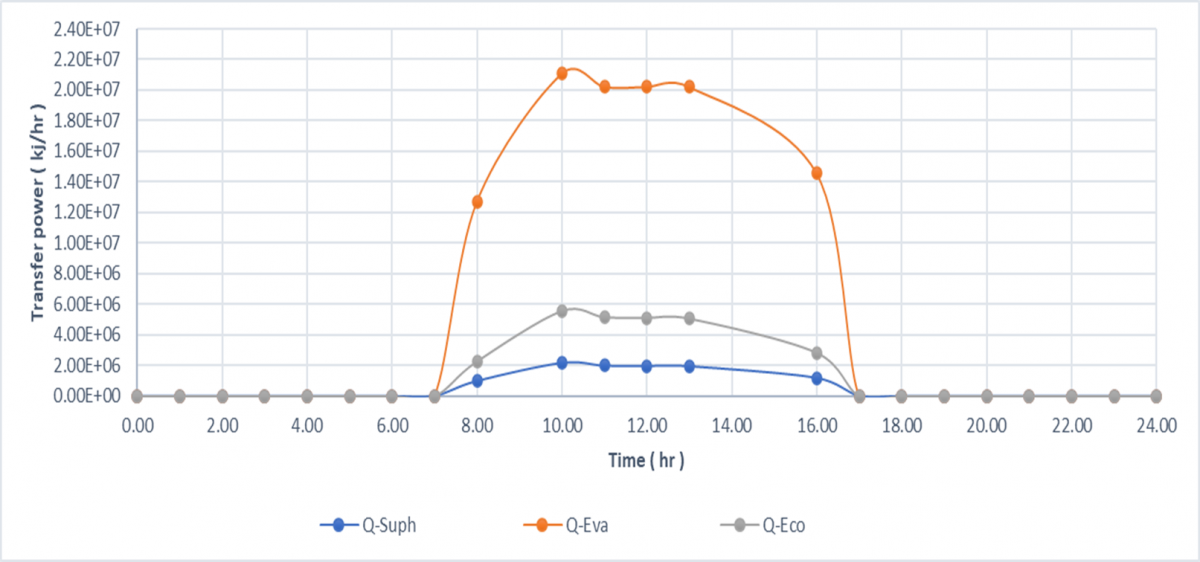
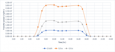
The curve presented in Figure 6a shows the transferred power obtained from each stage of the steam generator: superheater, evaporator, and economizer. The heat transferred to Qsup, Qeva, and Qec increases from 7:00 h (am) to a maximum value at 11:00 h (am), such that Qsup=1.99E+6 KJ/hr, Qeva=2.02E+7 KJ / hr, and Qeco=5.15E+6, then decreases to zero at 17: 00 h.

Figure 6b shows the evolution of the heat transferred on August 1 of each exchange, which indicates that the net heat transfer is higher than obtained on January 1. The heat transferred (Qsup, Qeva, and Qeco) goes into a rise from 5:00 h (am) and reaches a maximum value at 11: 00 h (am) such that Qsup=6.86E+6 KJ/hr, Qeva=3.71E+7KJ/hr and Qeco=1.76E+7, then declines in the next period to reach a zero value at 19: 00 h.

6a.png

(a)

6b.png

(b)

Figure 6. Transferred power variation (a) during the Day of January 1, (b) during the Day of August 1

The reason for the variation in the values between January and August is that the solar appearance period in the summer is longer than in winter, and the amount of solar radiation falling is higher in summer and this directly affects the temperatures outside of the boiler. This affects the amount of power output, which is explained by the following equation:

$\mathrm{Q}_{\text {trans }}=\mathrm{m}_{\text {hot }} * \mathrm{cp}_{\text {hot }} *\left(\mathrm{~T}_{\text {hot.in }}-\mathrm{T}_{\text {sat }}\right)$      (1)

4.4 The steam turbine work

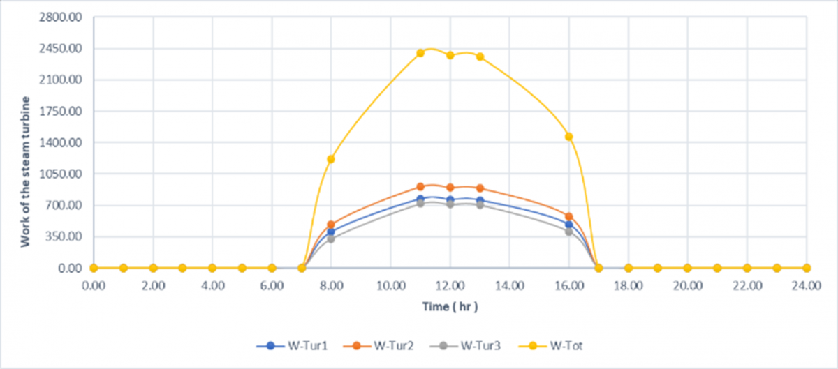
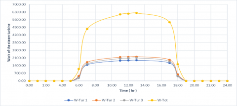
Figure 7a and b depict the variation in work obtained by the steam turbine in this simulation on January 1 and August 1. On January 1, the work begins to increase at 7:00 a.m. and continues until it reaches a maximum value of 2399 kJ/kg at 11:00 a.m., which corresponds to both heat exchange and steam-generated power. Then it decreases until it reaches zero at 17:00 h. On August 1, the work began to increase from 5:00 a.m. to a value of 6084 kJ/kg at 11:00 a.m. Then it decreases after this maximum value, so that it is zero at 19:00 h.

The reason for the variation between January and August, besides the previous reasons mentioned before, is that the steam exiting from the superheater in Augusta has a higher enthalpy than it does in January. Steam with higher enthalpy achieves more expansion and a higher power net, corresponding to the temperature difference.

$\mathrm{W}_{\mathrm{Tur}}=\mathrm{m}\left(\mathrm{h}_{\mathrm{o}}-\mathrm{h}_{\mathrm{i}}\right)$     (2)

A specific thermodynamic simulation of PTC uses TRANSYS software in order to simulate the performance during part-load conditions. In this design-model, the technical outcomes were used to back-calculate Rankine turbine efficiency and the heat exchangers.

The results showed that the PTC improves the overall solar field efficiency, the ability of PTCC to absorb both diffuse irradiance of solar and. Also, the PTC is used for high power capacity installations as its efficiency is high in the low-medium temperature ranges. This result is in close agreement with [35, 36].

7a.png

(a)

7b.png

(b)

Figure 7. Work (kJ/kg) variation of the steam turbine (a) during the Day of January 1, (b) during the Day of August 1

The working fluid and HTF are selected based on specific criteria: heat transfer, evaporation - temperature and temperature range [34]. The THERMINOL VP-1 and water were chosen as the best HTF and working fluid for the solar field and the three-stage Rankine cycle. results showed that the location of the site, hour number and highest solar radiation permit the positive gain of heat in the solar field and high energy production, and this is the same result obtained by most studies in the literature [32, 37, 38]. It is obvious that the temperature variations of the inlet and outlet of the PTC and heat exchanger are affected by weather variations and consequently affect the power generated from the steam turbine (LP, IP, and HP stage). It is clear that the average temperature is higher than in winter and so the generated power is higher in summer.

Moreover, the results showed that in August, compared to January, the decrease in solar radiation is 48% and the reduction in the PTC heat gain is 58%, resulting in a decrease in the power produced by the steam turbine of 67%. These results are slightly similar to the results which were obtained by Rohani et al. [39]. Furthermore, the results show that the PTC yield guarantee covers the Rankine cycle heat input, which necessitates a large area.

This simulation is applicable throughout the year and through the establishment of an integrated power plant for the production of electricity from solar energy, with the possibility of storing the excess energy with the adoption of a larger area of the solar field via solar batteries.