Atif Laiche* | Allaoua Boulahia
© 2022 IIETA. This article is published by IIETA and is licensed under the CC BY 4.0 license (http://creativecommons.org/licenses/by/4.0/).
OPEN ACCESS
Flexible structures outperform rigid ones thanks to their lightweight, dexterous maneuverability as well as their suitability towards high vibration. To this end, a rectangular-shaped wing is modeled as a flexible cantilever beam under two loading conditions, namely the former is a uniformly distributed force which is triggered by gravity while the latter is a tip load. In the same context, this paper addresses the lumped parameter method (LPM) for modeling a flexible wing using SimMechanics (also called Simscape Multibody) and Simulink environment by considering the wing as a concatenation of small elements connected together through springs and dampers. To verify the proposed model, simulation examples are carried, from which it is found that the simulation results approximately match the analytical findings. To emphasis, comparatively speaking, the obtained results from SimMechanics model provides with the same results as in modal analysis which is performed through Ansys workbench, namely the achieved deflection as well as modes shape from the conventional formulas fit in with the deflection obtained from the developed model in SimMechanics.
modeling, lumped parameter approach, finite element analysis, wing deflections, oscillations, static deflection, Simscape multibody, Simulink
The utility of flexibility in mechanical structures plays an important role when it comes to dealing with structures subjected to substantial loads. Basically speaking, from a theoretical point of view, SimMechanics and Simulink are widely used to model flexible dynamics. Many researchers shifted towards using SimMechanics and Simulink to grasp the behavior of a wide range of structures. For instance, Victor et al. [1] have used lumped parameters and finite element method to model and predict the beam’s deflection in a linear regime, in which they have compared both methods to find out that the lumped parameter is a user-friendly approach to be implemented for flexible bodies yet it has drawbacks which are shown when it comes to modeling high dimensional structures. In the work developed by Subedi et al. [2], a flexible beam is experimentally modeled using a camera to identify the lumped parameters of a flexible structure. This experience showed that an increasing number of elements reduces the deflection’s ratio. In Ref. [3], a model has been developed based on the port Hamiltonian formulation and applied to a robotic system.
In the field of robotics, the lumped parameter method has found its place in modeling robots and machine tools which perform at high speed [4]. In the study [5], a new method which minimizes the impact of vibration is proposed and applied on a rigid structure which aims at subdividing the whole structure into separated elements.
A flexible fishing rod model is used to model a single-link flexible manipulator through LPM-based SimMechanics [6]. From the study [7], a survey of the literature related to dynamic analyses of flexible robotic manipulators has been carried out. In Ref. [8], the global shape functions for flexible multibody systems can be obtained using isogeometric finite element models which aim at discretizing the geometry. Flexible multibody systems software is developed by Held et al. [9] in Matlab toolbox Dynmanto, to incorporate flexible bodies in multibody simulations, the global shape functions for flexible multibody systems can be obtained using isogeometric finite element models which aims at discretizing the geometry. The usefulness of the lumped parameter method is introduced in Refs. [10, 11], and it is an effective method for predicting the contact force of elastic colliding bodies. In addition, the advantages of this method are in its simplification of mathematical formulation, computational efficiency, and better understanding of the coupling effect of the excited modes on the occurrence of multiple impacts. From the work [12], an improved approximation is presented to calculate wing tip deflection. It is very well suited for preliminary designs of wings. According to Hatch [13], A literature study which aims to practical the different methods of constructing, representing dynamic mechanical models and develop a strong understanding of modal analysis, where the total response of a system can be constructed by combinations of the individual modes of vibration. The lumped parameter method has been proved efficient in a wide range of domains such as acoustics and mechanics [14]. In the work developed by Svoboda and Hromčík [15], the finite element based structural model of a flexible wing is presented, in which the problem is addressed using Euler-Bernoulli. This method shows a remarkable accuracy towards modeling. Mathematical modeling and simulation analysis of aerodynamic loads act on the wing structure namely the aerodynamic lift, load due to the weight of the wing and load due to the fuel stored in wing are presented in Ref. [16]. This study is made through Matlab and the developed model analytically points out the critical parameters that influence the system’s behavior. Additionally, numerical analysis is carried out using finite element analysis to obtain pressure distribution, von mises stress and displacement of the wing structure. However, very few works have addressed the wing’s deflection using lumped parameters through Matlab and Simulink. To this end, in this paper, a lumped parameter method is applied on a rectangular wing to assess the wing’s behavior when subjected to different load types. The rest of the paper is organized as follows: section 2 deals with modeling of the wing. In section 3, simulation analysis is carried out using Matlab and Simulink. Finally, this paper concludes with the most important findings and the potential future work regarding this work.
2.1 Modeling of a flexible rectangular wing using LPM
A wide range of methods have been developed to study the behavior of flexible bodies and SimMechanics is one of the handy tools to grasp this behavior. In this work, an application of the Lumped parameter approach is used to model a rectangular wing. Basically, the lumped parameters approach consists of modeling the structure as a set of elements, which are connected through springs (k) and dampers (b) as it is shown in Figure 1.
Figure 1. A flexible body according to the lumped-parameter method [17]
The main idea of modeling a rectangular wing fixed-free with S1223 airfoil cross-section is depicted in Figure 1. The wing is approximated as a collection of discrete flexible units fixed to one another through welding (W) in order to ensure the best connection between units. In reality, the welding (W) replaces the wing's ribs. The coupled units effect affects structure strength. Furthermore, connect the rigid connections between the flexible unit to construct a complete flexible body. For each type of deformation represented, each flexible wing unit provides one internal degree of freedom to the body. The model is completed by the body's boundary conditions, which are imposed by joints, kinematic restrictions, or explicit forces and torques. Each flexible unit is composed of two rigids body elements named (m1, m2) connected through a revolving joint block involving internal springs (k) and dampers (b) to capture its stiffness and damping characteristics to obtain a compliant behavior [1]. Furthermore, the SimMechanics-based model is shown in Figure 2.
Figure 2. Simscape Multibody diagram of a flexible wing unit (one element)
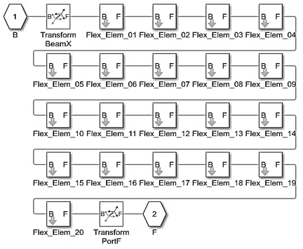
Figure 3. Simscape Multibody model of wing with twenty subsystems
The flexible joint aims at joining two bodies with one rotational degree of freedom which itself provides a motion to the base (B) and follower (F) according to a single time-varying transformation. The base (B) and follower (F) have a reciprocity movement which keeps the frame's origins coincident throughout the simulation. The main role of one of the revolutionary primitives is to offer a rotational degree of freedom. This transformation is applied by the primitive Pz, making the follower frame rotate according to the base frame.
The model in Figure 3 shows the generic structure of the wing. A chain of flexible elements connects frames B and F which are the ports of the block. The number of elements can be varied.
2.2 Description of the Simulink model
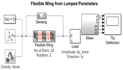
The model in Figure 4 shows a flexible wing modeled using the lumped parameter method.
Figure 4. Simscape Multibody model of the complete system
The various blocks connect to each other and to the world frame. Flexible wing block contains the necessary elements to build the LPM such as material properties, damping factor, geometry of the wing, number of elements and flexibility type. From load’s block we can apply an external force and torque at the attached frame. The force and torque are specified by the physical signal inputs. Sensor block is used to detect the deflections of the interface frames in relation to the flexible body model's frames. The sensing signals (position, velocity, acceleration) are important as inputs to the deformation model. Transient simulations can be used to determine the static deflection of the wing due to gravity. A force can also be applied to the tip of the wing.
This model is configured so that linearization techniques can be used to identify the different natural frequencies of the wing at various modes [17].
A rectangular wing is represented in Figure 5. One end of the wing is fixed at the root, while the other end at the tip is free.
Figure 5. (a) 3D Wing model; (b) 2D Airfoil shape
The considered wing’s parameters are defined in Table 1.
Table 1. Wing dimensions, moment of inertia and material properties
|
Length (L) |
0.3 (m) |
|
|
Chord length (C) |
0.1 (m) |
|
|
Area cross-section (A) |
8.2178.10-4(m4) |
|
|
Area moment of inertia (Ixx) |
6.8030.10-9(m4) |
|
|
Area moment of inertia (Iyy) |
1.9067.10-6(m4) |
|
|
Torsion J |
2.6662.10-8(m4) |
|
|
Aluminum Material |
Material Density ρ |
2800 (kg/(m3)) |
|
Modulus of Elasticity (E) |
70.103 (MPa) |
|
|
Shear Modulus (G) |
27.103 (MPa) |
|
2.3 Spring coefficient
From a mathematical point of view, the stiffness (k) of the revolute joint is calculated by the following formula.
$k=\frac{E \cdot I}{l}[\mathrm{Nm} / \mathrm{rad}]$ (1)
If the flexible wing has length L and a number n of flexible wing units, then the length ℓ of an undeformed flexible wing unit is simply.
$l=\frac{L}{n}[m]$ (2)
2.4 Damping coefficient
The Damping of the wing is specified by two damping factors. The two factors enable the damping to scale with the dimensions and material used in the wing. When density of material increases, damping Ratio also increases and natural frequency decreases.
The damping coefficient C used in the flexible elements is calculated according to the following formulas:
$C_{\text {bending }}=f_{\text {elastic }} \cdot \frac{E \cdot I}{l}\left[\frac{N m}{\left(\operatorname{rad~sec}^{-1}\right)}\right]$ (3)
$C_{\text {bending }}=f_{\text {elastic }} \cdot \frac{E \cdot A}{l}\left[\frac{N m}{\left(\operatorname{rad~sec}^{-1}\right)}\right]$ (4)
$C_{\text {torsion }}=f_{\text {shear }} \cdot \frac{E . J}{l}\left[\frac{N m}{\left(\mathrm{rad} \mathrm{sec}^{-1}\right)}\right]$ (5)
Simulations of the considered model are carried out through the Matlab environment and the obtained results are discussed in the following sections.
3.1 Validation of static deflection
The static deflection for a cantilever beam can be calculated using Euler-Bernoulli beam theory. The bending moment, shear force and wing deflection can be figured out using mathematical axioms dedicated to engineering beam applications.
In this case, a rectangular wing can be regarded as a beam, so the analytical deflection has been calculated using Eq. (6).
$\delta=\frac{q . L^{4}}{8 . E . I}=0.0048[m]$ (6)
$q=\rho \cdot A \cdot g=2.257310^{3}\left[\frac{N}{m}\right]$ (7)
where, q is the uniformly distributed load on the beam (force/unit length). We have multiplied the gravity by 100 for the sake of clearly showing the wing’s deflection since it takes negligible values. By substituting the value of q into Eq. (6) the deflection is δ=0.0048 [m].
The remaining parameters used in Eq. (6) are previously defined in Table 1. From the simulated model, the ‘δ’ value is found to be, δ=0.0047 [m].
Figure 6. Static deflection from lumped parameter model
From Figure 6, the comparison between the tip deflection of the wing modeled is graphically presented using a lumped parameter as the number of elements is varied. The results of transient simulations closely match theory, especially as the number of elements grows.
3.2 Loads types
Case I: Distributed load (Loaded under self-weight)
In this section, the wing is exclusively subjected to its own weight.
As it is shown in Figure 7, the vertical deflection of the wing tip is plotted versus time. The wing lightly oscillates from a range of [0 0.095 m] until it takes an equilibrium state at δ=0.00479 m after approximately 1.5 seconds.
Figure 7. Vertical deflection of wing tip
Case II: Tip load
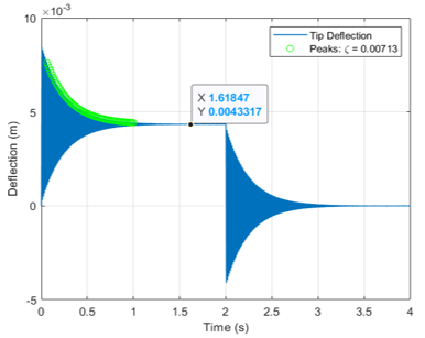
Differently to the previous simulation, the wing is subjected to a tip load of 230 N then it is released after 4 seconds. After releasing it, the wing oscillates from [0 0.0075 m] until it takes an equilibrium state at δ=0.0043 m as shown in Figure 8. The peaks are used to calculate the damping ratio ξ.
Figure 8. Vertical deflection of wing tip
The analytical deflection at the free end of the wing is calculated using Eq. (8).
$\delta=\frac{F . L^{3}}{3 . E . I}=0.0043[\mathrm{~m}]$ (8)
where, F=230[N].
Using Eq. (8), the obtained value of vertical deflection is found to be: δ=0.0043 [m].
The damping ratio can be found from the logarithmic decrement [17].
$\xi=\frac{1}{\sqrt{1+\left(\frac{2 . \pi}{\delta}\right)^{2}}}$ (9)
3.3 Comparison of elements’ deflection
In this simulation example, a variety of elements are used to describe the wing’s structure, namely the wing takes 10, 20 and 30 elements in order to point out the effect of an increasing number of elements.
Figure 9. Effect of number of flexible elements in LPM
In this study, it is not necessary to be limited to a number of elements lower than 10 because it is also necessary to think about topic optimizations and it is necessary to know how far an element can go in order to attenuate the amplitudes of the vibrations. Comparatively speaking, the three graphs of 10, 20 and 30 elements respectively in Figure 9 show similar oscillations’ values. However, the increment of elements paves the way to minimizing the wing’s deflection. The relationship between the number of elements and the wing’s deflection is an inverse relationship. So, it can be concluded from Figure 9, as the number of elements increase, the wing lightly oscillates. Approximately, the best way to minimize the deflection of the wing is to increase the number of elements more than 10 elements.
3.4 Mode shape
The different natural frequencies of the modes' shapes are calculated using linearization. The natural frequencies can be predicted using the theoretical Eq. (10).
$\omega_{n}=\frac{\beta_{n} \cdot \sqrt{\left(\frac{E . I}{\rho . A}\right)}}{L^{2}}$ (10)
For the boundary conditions in this model (fixed-free), βn = [3.52 22 61.7 121].
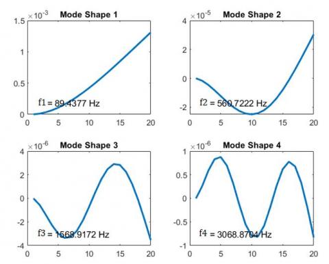
It is noteworthy to say that the previously existing formulas for deflection properly fit in with the simulated wing model. In other words, the analytical deflection values are in a good match with the simulation wing’s deflection Figure 10 shows the first mode shapes of the wing which are obtained from LPM in Matlab code. In this figure, mode shape 1, represents the first bending mode of the wing with lower natural frequency. Remarkably, mode shape 4 has a higher natural frequency as well as torsional mode. The other modes, namely mode shape 2 and 3 have lower frequencies and often higher amplitudes; thus, the lower modes are more dominant than the higher modes. For this reason, higher modes are usually neglected in the LPM and the modal approach.
Figure 10. First four mode shapes
From a comparison point of view, a second method was made through Ansys Software in order to validate once again the model used in section (2). Structural and Modal analysis are performed using the Finite Element Method to obtain the total deformation and different modes of the wing. Automatic algorithms are built in these software packages to automatically extract the required information for pre- post processing.
In Table 2, a comparison study of the obtained deflection from analytical calculation, LPM and Ansys software is made in order to confirm once again the small deflection of the wing structure.
Table 2. Comparison study of the obtained deflection from analytic, Matlab and Ansys
|
|
Equilibrium deflection (analytic) |
Lumped parameter simulations |
Finite element simulations |
|
Self-weight |
0.0048 [m] |
0.0047 [m] |
0.00456[m] |
|
Tip load |
0.0043[m] |
0.0043 [m] |
0.00428[m] |
For comparison, Table 3, resumes the different values of the vibration frequencies of mode shapes which are obtained from analytical theory, lumped parameter method and Ansys software. In order to obtain a similar value of the vibration frequencies, we choose the concatenation of 20 elements of the wing structure in the LPM.
Table 3. Comparison study of mode shapes obtained from analytical theory, lumped parameter method and finite element analysis
|
Approaches |
Vibration frequency [Hz] |
|||
|
Analytical Calculations |
89.54 |
560.72 |
1535.20 |
2866.90 |
|
LPM (20 Elements) |
89.43 |
560.72 |
1568.91 |
3068.87 |
|
FEA Software |
91.54 |
562.02 |
1535.2 |
2866.9 |
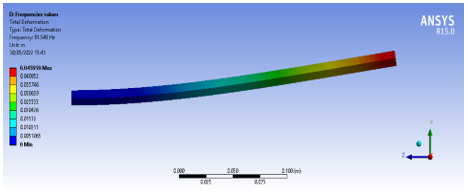
Figure 11. Vertical deflection of wing tip
Obviously, as it is shown in Figure 11, the most influenced zone is labeled by red color which is located at the wing’s tip and that due to the force’s location for the case of tip load (refer to Figure 11(b)). However, the second case depicts the deformation of the wing when subjected to its self-weight (refer to Figure 11(a)).
Figure 12. Comparison of modes shape
Comparatively speaking, in Figure 12, a comparison study of the different natural frequencies is carried out using both methods. Both curves show that the different natural frequencies obtained from Matlab code are in a good match with those obtained from Ansys software.
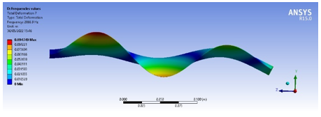
Similarly, to Figure 10, Figures 13-16 represent the first mode shapes obtained from finite element model. To emphasize, the previously achieved mode shapes using LPM perfectly conduct to the same results from finite element method in terms of natural frequencies and mode shapes form.
Figure 13. First mode shape
Figure 14. Second mode shape
Figure 15. Third mode shape
Figure 16. Fourth mode shape
In this paper, the obtained results from SimMechanics model provides with the same results as in finite element analysis which is performed through Ansys workbench, namely the vertical deflection as well as mode shapes from the conventional formulas fit in with the deflection obtained from the developed model in SimMechanics. In other words, the previously existing formulas for deflection properly fit in with the simulated wing model. The analytical deflection values are in a good match with the simulation wing’s deflection.
As the number of discrete elements is varied, the lumped parameter method gives accurate results for static bending, yet the finite element analysis provides more accurate results for vibration modes, frequencies and time consumption.
It can be concluded that the application of the lumped parameter approach through Matlab and Simulink is a reliable approach to describe the behavior of flexible bodies.
The potential future work resides in using a state-space method based on finite element analysis through Matlab and Simulink in order to compare it with the lumped parameter method.
[1] Victor, C., Kennedy, D., Arnav, M., Jeff, W. (2006). Modeling flexible bodies in Simmechanics and Simulink. Mathworks, 1: 1-6.
[2] Subedi, D., Tyapin, I., Hovland, G. (2020). Modeling and analysis of flexible bodies using lumped parameter method. In 2020 IEEE 11th International Conference on Mechanical and Intelligent Manufacturing Technologies (ICMIMT), Cape town, South Africa, pp. 161-166. http://dx.doi.org/10.1109/ICMIMT49010.2020.9041188
[3] Macchelli, A., Melchiorri, C., Stramigioli, S. (2007). Port-based modeling of a flexible link. IEEE Transactions on Robotics, 23(4): 650-660. http://dx.doi.org/10.1109/TRO.2007.898990
[4] Khalil, W., Gautier, M. (2000). Modeling of mechanical systems with lumped elasticity. Proceedings 2000 ICRA. Millennium Conference. IEEE International Conference on Robotics and Automation. Symposia Proceedings (Cat. No. 00CH37065), 4: 3964-3969. http://dx.doi.org/10.1109/ROBOT.2000.845349
[5] Yushu, B., Zhihui, G., Yuchun, D. (2013). Impact vibration reduction for flexible manipulators via controllable local degrees of freedom. Chinese Journal of Aeronautics, 26(5): 1303-1309. https://doi.org/10.1016/j.cja.2013.04.010
[6] Patra, S., Sarkhel, P., Hui, N.B., Banerjee, N. (2020). Modelling and simulation of a fishing rod (Flexible Link) using Simmechanics. Journal Européen des Systèmes Automatisés, 53(4): 451-460.
[7] Gaultier, P.E., Cleghorn, W.L. (1989). Modeling of flexible manipulator dynamics: A literature survey. In Proc of 1st Natl App Mech and Robotics Conf.
[8] Rückwald, T., Held, A., Seifried, R. (2022). Flexible multibody impact simulations based on the isogeometric analysis approach. Multibody System Dynamics, 54(1): 75-95. http://dx.doi.org/10.1007/s11044-021-09804-x
[9] Held, A., Moghadasi, A., Seifried, R. (2020). DynManto: A Matlab toolbox for the simulation and analysis of multibody systems. International Design Engineering Technical Conferences and Computers and Information in Engineering Conference, 83914, V002T02A005. http://dx.doi.org/10.1115/DETC2020-22336
[10] Lee, Y., Hamilton, J.F. (2015). The lumped parameter method for elastic impact problems. Journal of Applied Mechanics, 50(4a): 823-827. https://doi.org/10.1115/1.3167152
[11] De Lannoy, S. (2014). Wing bending calculation with a single set of equations. Wingbike-A Human Powered Hydrofoil, 1-17.
[12] Wang, Y., Huston, R.L. (1994a). A lumped parameter method in the nonlinear analysis of flexible multibody systems. Computers and Structures, 50(3): 421-432. http://dx.doi.org/10.1016/0045-7949(94)90011-6
[13] Hatch, M. (2000). Vibration simulation using MATLAB and ANSYS. https://doi.org/10.1201/9781420035759
[14] Jiang, Y.W., Xu, D.P., Jiang, Z.X., Kim, J.H., Hwang, S.M. (2019). Comparison of Multi-physical coupling analysis of a balanced armature receiver between the lumped parameter method and the finite element/boundary element method. Applied Sciences, 9(5): 839. https://doi.org/10.3390/app9050839
[15] Svoboda, F., Hromčík, M. (2017). Finite element method based modeling of a flexible wing structure. In 2017 21st International Conference on Process Control (PC), pp. 222-227.
[16] Laiche, A., Boulahia, A. (2022) Modeling and simulation analysis of aircraft wing loads. International Journal of Advanced Research in Engineering and Technology, 13(5): 32-39. https://doi.org/10.17605/OSF.IO/N42SB
[17] Miller, S., Soares, T., Weddingen, Y., Wendlandt, J. (2017). Modeling flexible bodies with Simscape multibody software. Technical Paper. www.mathworks.com/content/dam/mathworks/tag-team/Objects/s/Modeling-Flexible-Bodies-Simscape-Multibody-171122.pdf.