Huthaifa Al-Khazraji
© 2022 IIETA. This article is published by IIETA and is licensed under the CC BY 4.0 license (http://creativecommons.org/licenses/by/4.0/).
OPEN ACCESS
This paper presents a Proportional-Derivative State Feedback (PDSF) controller approach to design an active suspension system for quarter car. The objective of the PDSF controller is to eliminate the effects of road disturbances to achieve ride comfort of the driver and passengers. Finding the optimal feedback gain matrix of the PDSF controller is formulated as an optimization problem. Then, two meta-heuristic optimizations named Bees Algorithm (BA) and Grey Wolf Optimization (GWO) are employed to optimize the feedback gain matrix of the PDSF controller based on the Integral Time of Absolute Error (ITAE) index. The results show the superiority of the BA-based PDSF controller in terms of reducing the ITAE index in comparison with the results obtained from GWO based PDSF.
proportional-derivative state feedback controller, suspension system, meta-heuristic optimization, bees algorithm, grey wolf optimization
Suspensions systems have been widely studied in the literature. The main objective of the suspension system is to isolate the car body from road disturbances [1]. The suspension systems can be categorized broadly as passive, semiactive and active. In the passive suspension system, a conventional method by utilizing a spring and a damper is used. The passive suspension system cannot handle the changes in road conditions [2]. In the case of a semiactive suspension system as compared to the passive suspension system, the conventional damper is replaced by a controllable damper. However, the active suspension system has an actuator parallel with the damper and the spring to improve passenger comfort [3]. The objective of the actuator is to reduce the vertical force that is transmitted to the car body by designing a suitable controller.
Various controller strategies for active suspensions systems have been designed and investigated to ensure better ride comfort. For example, Sam et al. [4] presented a controlling strategy based on Proportional-Integral Sliding Mode Control (PI-SMC) for active suspensions systems. Kumar and Vijayarangan [5] developed a Linear Quadratic Controller (LQR) active suspensions system for 3 degrees of freedom quarter car. The performance of the LQR active suspensions system is compared with the passive suspensions systems based on the Root Mean Square (RMS) index. The results show the superiority of the LQR active suspensions system. A robust control based on Sliding Mode Control (SMC) that allows avoiding the road disturbance for a quarter-car suspensions system is proposed by Alvarez-Sánchez [3]. The mass of the quarter-car was estimated using an algebraic estimator based on the identification method. Yakub et al. [6] presented a comparative study between the Proportional-Integral-Derivative (PID) controller and State Feedback (SF) controller to design a quarter car suspension system. The outcomes of this study show that the vibration in the suspension system has been significantly improved by using the SF controller as compared to the PID controller.
Due to the usefulness of using optimization techniques instead of try and error method, many authors prefer to utilize meta-heuristic optimizations to determine the optimal tuning parameters of the controller. In this direction, Nagarkar and Vikhe [7] optimized the weighting matrix of the LQR controller using a Genetic Algorithm (GA). The performance of the GA-LQR controller for the quarter car suspension system is evaluated based on the RMS index. Romsai et al. [8] presented an application of tuned the designed parameters of the PID controller using Lévy-fight intensified current search (LFICuS) to improve the performance of the active suspension system. Parallel to these studies, this paper aims to investigate the ability of two meta-heuristic optimizations, Bees Algorithm (BA) and Grey Wolf Optimization (GWO), to optimize the feedback gains matrix of the Proportional-Derivative State Feedback (PDSF) controller based on Integral Time of Absolute Error (ITAE) index. The simulation results indicate that tuning the PDSF by BA was able to reduce the ITAE by 14.3% in comparison with tuning the PDSF by GWO.
The arrangement of the paper is as follows. Section 2 presents the dynamic modeling of the active suspension system. The PDSF controller is introduced in Section 3. Section 4 explains the two meta-heuristic optimizations. The simulation results are given in Section 5. Lastly, Section 6 will summarize the conclusion of this paper.
In order to examine the impact of the design of a state feedback controller on the active suspension system on the quarter car, an accurate mathematical model of the system based on the state-space approach must be established. The two degrees of freedom (2DOF) active suspension system that is considered in this study is illustrated in Figure 1 [9] where ms (Kg) is the sprung mass (chassis) and mu (Kg) is the unsprung mass (wheel). An active suspension system can be represented as a passive suspension system with an actuator. The passive suspension system consists of a spring with a stiffness factor (ks) N/m and a damper with a damping factor (bs) Ns/m. A hydraulic actuator with force (Fa) N is added in parallel to the passive suspension. The tire has a stiffness factor (kt) N/m. The state variables of the system are the displacement (x1) m and (x2) m and velocity $\left(\dot{\mathrm{x}}_{1}\right) \frac{\mathrm{m}}{\mathrm{s}}$ and $\left(\dot{\mathrm{x}}_{2}\right) \frac{\mathrm{m}}{\mathrm{s}}$ of the sprung and unsprung mass respectively. The vertical displacement of the road (d) m is represented the road disturbance.
Figure 1. 2DOF active suspension system of the quarter car
Based on Newton’s laws, the equations of motion for the sprung mass are given by [8]:
$m_{s} \times \ddot{x}_{1}=-\left(k_{s} \times\left(x_{1}-x_{2}\right)\right)-\left(b_{s} \times\left(\dot{x}_{1}-\dot{x}_{2}\right)\right)+ \mathrm{F}_{\mathrm{a}}$ (1)
Rearrange of Eq. (1) yields:
$\ddot{\mathrm{x}}_{1}=-\left(\frac{\mathrm{k}_{\mathrm{s}}}{\mathrm{m}_{\mathrm{s}}} \times \mathrm{x}_{1}\right)+\left(\frac{\mathrm{k}_{\mathrm{s}}}{\mathrm{m}_{\mathrm{s}}} \times \mathrm{x}_{2}\right)-\left(\frac{\mathrm{b}_{\mathrm{s}}}{\mathrm{m}_{\mathrm{s}}} \times \dot{\mathrm{x}}_{1}\right)+\left(\frac{\mathrm{b}_{\mathrm{s}}}{\mathrm{m}_{\mathrm{s}}} \times \dot{\mathrm{x}}_{2}\right)+\left(\frac{1}{\mathrm{~m}_{\mathrm{s}}} \times \mathrm{F}_{\mathrm{a}}\right)$ (2)
In the same way, the equations of motion for the unsprung mass are given by [8]:
$\mathrm{m}_{\mathrm{u}} \times \ddot{\mathrm{x}}_{2}=\left(\mathrm{k}_{\mathrm{s}} \times\left(\mathrm{x}_{1}-\mathrm{x}_{2}\right)\right)+\left(\mathrm{b}_{\mathrm{s}} \times\left(\dot{\mathrm{x}}_{1}-\dot{\mathrm{x}}_{2}\right)\right)-\left(\mathrm{k}_{\mathrm{t}} \times\left(\mathrm{x}_{2}-\mathrm{d}\right)\right)-\mathrm{F}_{\mathrm{a}}$ (3)
Rearrange of Eq. (3) yields:
$\ddot{\mathrm{x}}_{2}=\left(\frac{\mathrm{k}_{\mathrm{s}}}{\mathrm{m}_{\mathrm{u}}} \times \mathrm{x}_{1}\right)-\left(\left(\frac{\mathrm{k}_{\mathrm{s}}}{\mathrm{m}_{\mathrm{u}}}+\frac{\mathrm{k}_{\mathrm{t}}}{\mathrm{m}_{\mathrm{u}}}\right) \times \mathrm{x}_{2}\right)+\left(\frac{\mathrm{b}_{\mathrm{s}}}{\mathrm{m}_{\mathrm{u}}} \times\right.\left.\dot{\mathrm{x}}_{1}\right)-\left(\frac{\mathrm{b}_{\mathrm{s}}}{\mathrm{m}_{11}} \times \dot{\mathrm{x}}_{2}\right)+\left(\frac{\mathrm{k}_{\mathrm{t}}}{\mathrm{m}_{\mathrm{u}}} \times \mathrm{d}\right)-\left(\frac{1}{\mathrm{~m}_{\mathrm{u}}} \times \mathrm{F}_{\mathrm{a}}\right)$ (4)
Based on Eq. (2) and Eq. (4) the state variable equations of the active quarter car suspension system are given by [8]:
$\left[\begin{array}{l}\dot{\mathrm{x}}_{1} \\ \ddot{\mathrm{x}}_{1} \\ \dot{\mathrm{x}}_{2} \\ \ddot{\mathrm{x}}_{2}\end{array}\right]=\left[\begin{array}{cccc}0 & 1 & 0 & 0 \\ -\frac{\mathrm{k}_{\mathrm{s}}}{\mathrm{m}_{\mathrm{s}}} & -\frac{\mathrm{b}_{\mathrm{s}}}{\mathrm{m}_{\mathrm{s}}} & \frac{\mathrm{k}_{\mathrm{s}}}{\mathrm{m}_{\mathrm{s}}} & \frac{\mathrm{b}_{\mathrm{s}}}{\mathrm{m}_{\mathrm{s}}} \\ 0 & 0 & 0 & 1 \\ \frac{\mathrm{k}_{\mathrm{s}}}{\mathrm{m}_{\mathrm{u}}} & \frac{\mathrm{b}_{\mathrm{s}}}{\mathrm{m}_{\mathrm{u}}} & -\frac{\left(\mathrm{k}_{\mathrm{s}}+\mathrm{k}_{\mathrm{t}}\right)}{\mathrm{m}_{\mathrm{u}}} & -\frac{\mathrm{b}_{\mathrm{s}}}{\mathrm{m}_{\mathrm{u}}}\end{array}\right] \times\left[\begin{array}{l}\mathrm{x}_{1} \\ \dot{\mathrm{x}}_{1} \\ \mathrm{x}_{2} \\ \dot{\mathrm{x}}_{2}\end{array}\right]+ \left[\begin{array}{c}0 \\ \frac{1}{\mathrm{~m}_{\mathrm{s}}} \\ 0 \\ -\frac{1}{\mathrm{~m}_{\mathrm{v}}}\end{array}\right] \times \mathrm{F}_{\mathrm{a}}+\left[\begin{array}{c}0 \\ 0 \\ 0 \\ \frac{\mathrm{k}_{\mathrm{t}}}{\mathrm{m}_{\mathrm{u}}}\end{array}\right] \times \mathrm{d}$ (5)
$\mathrm{y}=\left[\begin{array}{llll}1 & 0 & 0 & 0\end{array}\right] \times\left[\begin{array}{l}\mathrm{x}_{1} \\ \dot{\mathrm{x}}_{1} \\ \mathrm{x}_{2} \\ \dot{\mathrm{x}}_{2}\end{array}\right]$ (6)
In this paper, a Proportional-Derivative State Feedback (PDSF) controller is used to control the hydraulic actuator of the active suspension system. Consider the state-space model of a continuous Linear Time-Invariant (LTI) system with disturbance as follow [10]:
$\dot{\mathrm{x}}(\mathrm{t})=(\mathrm{A} \times \mathrm{x}(\mathrm{t}))+(\mathrm{B} \times \mathrm{u}(\mathrm{t}))+(\mathrm{W} \times \operatorname{dis}(\mathrm{t}))$ (7)
$y(t)=(C \times x(t))+(D \times u(t))$ (8)
where, $\mathrm{x}(\mathrm{t})$ and $\dot{\mathrm{x}}(\mathrm{t})$ are the states and the derivative states of the system. A, B, C and D are dynamic matrix, input matrix, output matrix and feedforward matrix of the system. u(t) is the control signal to the system whereas y(t) is the output [11]. Due to the presence of the disturbance, W is the disturbance matrix and dis(t) is the disturbance input.
In order to apply the PDSF controller, the states of the system need to be completely controllable and measurable. The basic idea of the PDSF controller is to measure the states of the system and to generate appropriate control action that regulates the system to achieve desirable performance. In the active suspension system, the objective of the controller is to regulate the states for any perturbation that happens in the road. The control action u(t) of the PDSF is selected as given in Eq. (9) [12]:
$\mathrm{u}(\mathrm{t})=-\left(\mathrm{k}_{\mathrm{p}} \mathrm{x}(\mathrm{t})\right)-\left(\mathrm{K}_{\mathrm{d}} \dot{\mathrm{x}}(\mathrm{t})\right)$ (9)
The control action u(t) of the PDSF controller represents the control force (Fa) N of the active suspension system, kp is the proportional gain matrix of the state feedback, Kd is the derivative gain matrix of the state feedback. Several approaches were used for finding the optimal feedback gain matrix of the PDSF controller [12]. To attain better control performance with less time consumption, two meta-heuristic optimizations named Bees Algorithm (BA) and Grey Wolf Optimization (GWO) are chosen for tuning the feedback gain matrix of the PDSF controller.
As mention above, the PDSF controller has tuning parameters that need to be adjusted to obtain the desired performance. Instead of using the trial and error method which is considered a time-consuming method, the tuning process in this study is formulated as an optimization problem. Then, two meta-heuristic optimizations, Bees Algorithm (BA) and Grey Wolf Optimization (GWO) are utilized to solve the problem.
4.1 Bees Algorithm
The Bees Algorithm (BA) is a swarm-based optimization algorithm developed by Pham et al. in 2005 [13]. The algorithm mimics the way that the honey bee when it is foraging for food. It consists of two methods of search: local search and random search. The optimization procedure of the BA begins with randomly initialized sites of a population of N scout bees within the search space as given in Eq. (10) [14]:
$p_{i}=p_{1}+\left(r \times\left(p_{u}-p_{1}\right)\right)$ (10)
where, pi is the initial site for each individual in the algorithm. i is the counter (i=1,2,3,…N). r is a round value generated between [0,1]. pl and pu are the lower and upper bounds of the search space of the problem.
Then, the objective value of each scout bee is evaluated. The next step is to select an elite bee (eli) based on the best objective value was found by the scout bees. After that, a number of sites (m) are selected to perform the local search. A local search towards the site of the elite bee (peli) is performed based on the patch size (h) as given in Eq. (11) [14]:
$p_{i}^{\text {new }}=p_{i}^{\text {old }}+h \times\left(p^{\text {eli }}-p_{i}^{\text {old }}\right)$ (11)
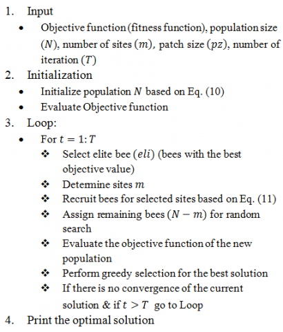
where, $p_{i}^{\text {new }}$ and $p_{i}^{\text {old }}$ are the new site and old site of the bee i respectively. The remaining bees (N-m) assign to search randomly as given in Eq. (10). The new population is evaluated and greedy selection is used for the best solution. The pseudo code of the BA is given in Figure 2.
Figure 2. Pseudo code of the BA
BA has been used by many authors as a controller-tuning technique. For example, Bilgic et al. [15] demonstrated the efficiency of the tuning of the LQR controller by using BA to stabilize an inverted pendulum. Moreover, Hameed et al. [16] presented a comparative study of tuning the parameters of the PID controller using BA and Firefly Algorithm (FA). Two different transfer functions were used in the study. Both algorithms achieve good dynamic performance when the system is subject to a step input.
4.2 Grey Wolf Optimization
Grey Wolf Optimization (GWO) is a swarm-based meta-heuristic optimization technique proposed by Mirjalili et al. in 2014. GWO simulates the social predatory behavior of gray wolves. Mirjalili et al. [17] categorized the individuals of gray wolves into four levels. The first category is the alpha wolf (α), these wolves either males or females are responsible to make decisions and lead the pack. The second category is the beta wolf (β), these wolves are lower level than the alphas which provide consultants to the alphas. The third category is the delta wolf (δ), these wolves submit information to alphas and betas. The last category is the omega wolf (ω) [18]. The simulation of the hunting process in GWO can be divided into three processes which are named: searching for prey, encircling prey and attacking prey. The general mathematical model of the movement of wolves towards the prey is formulated as follows [19]:
$C_{\mathrm{wo}}=2 \times r$ (12)
$A_{w o}=\left(2 \times a_{w o} \times r\right)-a$ (13)
$\mathrm{D}_{\text {wo }}=\left|\mathrm{C}_{\text {wo }} \times \mathrm{W}_{\text {wop }}(\mathrm{t})-\mathrm{W}_{\text {wo }}(\mathrm{t})\right|$ (14)
$\mathrm{W}_{\mathrm{wo}}(\mathrm{t}+1)=\mathrm{W}_{\mathrm{wop}}(\mathrm{t})-\left(\mathrm{A}_{\mathrm{wo}} \times \mathrm{D}_{\mathrm{wo}}\right)$ (15)
where, awo is a coefficient its value is linearly decreased from 2 to 0 for each iteration. Cwo, Awo and Dwo are coefficients their value are calculated as given in Eq. (12), Eq. (13) and Eq. (14) respectively. r is a random value generated between [0,1]. t refers to the current iteration in the algorithm. Wwop and Wwo are the position of the prey and the wolf respectively.
The hunting process is guided by the first three categories of wolves (α, β and δ). Hence, all wolves should adjust their position and movement based on the information that is provided by these three categories of wolves. The mathematical model of the hunting process can be represented as follows [17]:
The movement of individual wolf with respect to alphas α :
$\mathrm{D}_{\mathrm{wo \alpha}}=\left|\left(\mathrm{C}_{\text {wo1 }} \times \mathrm{W}_{\mathrm{wo \alpha}}\right)-\mathrm{W}_{\mathrm{wo}}(\mathrm{t})\right|$ (16)
Wwo1=Wwoα-(Awo1×Dwoα) (17)
The movement of individual wolf with respect to betas β:
$\mathrm{D}_{\mathrm{wo} \beta}=\left|\left(\mathrm{C}_{\mathrm{wo} 2} \times \mathrm{W}_{\mathrm{wo} \beta}\right)-\mathrm{W}_{\mathrm{wo}}(\mathrm{t})\right|$ (18)
$W_{\mathrm{wo} 2}=W_{\mathrm{wo} \beta}-\left(A_{\mathrm{wo} 2} \times \mathrm{D}_{\mathrm{wo} \beta}\right)$ (19)
The movement of individual wolf with respect to deltas δ:
$\mathrm{D}_{\mathrm{wo \delta}}=\left|\mathrm{C}_{\mathrm{wn} 3} \cdot \mathrm{W}_{\mathrm{wo \delta}}-\mathrm{W}_{\mathrm{wo}}(\mathrm{t})\right|$ (20)
$W_{\mathrm{WO} 3}=W_{\mathrm{wo} \delta}-\left(A_{\mathrm{wo} 3} \times \mathrm{D}_{\mathrm{wo} \delta}\right)$ (21)
The new position of individual wolf:
$W_{\text {wo }}{ }^{N e w}(t+1)=\frac{W_{\text {wo1 }}+W_{\text {W02 }}+W_{\text {wo3 }}}{3}$ (22)
where, Wwoα, Wwoβ and Wδwo are the best solution found by alpha, beta and delta respectively. The Pseudo code of the GWO algorithm is given in Figure 3. In the context of control engineering, it has been observed that the GWO is successfully handling the tuning process of the parameters of controllers in a number of papers such as for Proportional-Integral (PI) controller [19], Proportional-Integral-Derivative (PID) [20], and Fractional Order PID (FOPID) controller [21].
Figure 3. Pseudo code of the GWO
This section presents simulations of the PDSF controller approach to design an active quarter car suspension system. The Matlab software is used to conduct simulations and analyze the performance. The parameters of the quarter car suspension system are selected as given in Table 1 [8].
Table 1. Quarter car active suspension system parameters
|
Parameters |
Symbol |
Values |
Units |
|
Sprung mass |
ms |
300 |
Kg |
|
Unsprung mass |
mu |
60 |
Kg |
|
Stiffness of sprung spring |
ks |
16000 |
N/m |
|
Stiffness of tire spring |
kt |
19000 |
N/m |
|
Damping factor of sprung damper |
bs |
1000 |
Ns/m |
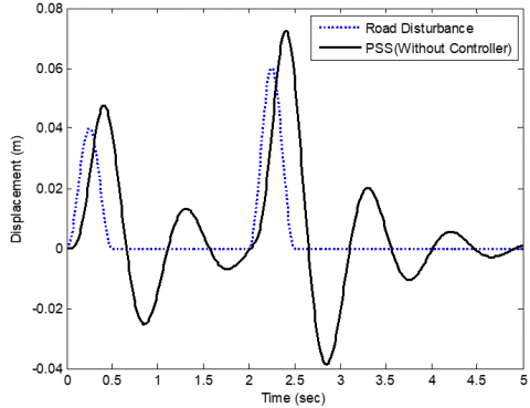
Initially, the performance of the Passive Suspension System (PSS) was tested to a road disturbance. The simulation was performed for a period of 5 seconds. The profile of the road disturbance d was chosen as a double bump in the form of:
d=$\left\{\begin{array}{cl}\gamma_{1} \times\left(1-\cos \left(4 \times \pi \times \mathrm{t}_{\mathrm{sim}}\right)\right), & 0 \leq \mathrm{t}_{\operatorname{sim}} \leq 0.5 \\ \gamma_{2} \times\left(1-\cos \left(4 \times \pi \times \mathrm{t}_{\mathrm{sim}}\right)\right), & 2 \leq \mathrm{t}_{\mathrm{sim}} \leq 2.5 \\ 0, & \text { otherwise }\end{array}\right.$ (23)
where the value of γ1 and γ2 were chosen to be 0.02 and 0.03 to simulate bumps with height of 0.04 m and 0.06 m.
The investigation of the dynamic performance of the PSS is presented in Figure 4. Figure 4 shows that the system has an oscillation frequency response (unstable). Therefore, an Active Suspension System (ASS) using an optimal PDSF controller based on BE (BE-PDSF) and GWO (GWO-PDSF) are implemented to improve the dynamics of the suspension system. The Integral Time of Absolute Errors (ITAE) criterion was selected as a cost function for the BA and the GWO to tune the feedback gain matrix of the PDSF controller. The ITAE is given by [22]:
ITAE $=\int_{0}^{t} \operatorname{sim} t_{\operatorname{sim}} \times|e(t)| d t$ (24)
where, tsim denotes the period time of the simulation and e is the error between the displacement of the sprung mass x1 and the initial value (i.e. zero). Therefore, the optimization problem for the PDSF controller approach to design an active suspension system for the quarter car is defined as:
minimize $\{$ ITAE $($ var $)\}$ (25)
where, ITAE is the objective functions that need to be minimized. The decision vector var is the four proportional feedback gain matrix for each state and one derivative feedback gain of the output of the PDSF controller.
Figure 4. Road disturbance profile
The parameters of the BA and GWO algorithms are given in Table 2. These values are obtained experimentally. The experiments are performed repeatedly until the solution quality of both algorithms is improved. The simulations are carried out for BA- PDSF and GWO- PDSF models as shown in Figure 5. The performance measured in terms of ITAE is summarized in Table 3. The set of the controller's parameters for both BA- PDSF and the GWO- PDSF controlled system are given in Table 4.
Table 2. BA and GWO algorithms parameters
|
Parameters |
BA |
GWO |
|
Number of population (N) |
50 |
50 |
|
Number of iteration (T) |
100 |
100 |
|
Patch size (h) |
2 |
- |
|
Number of sites (m) |
10 |
- |
|
Coefficient value (a) |
- |
2 |
Table 3. Performance comparison between BA-PDSF and GWO-PDSF
|
Performance Index |
BA-PDSF |
GWO-PDSF |
|
TIAE |
0.24 |
0.28 |
Table 4. Set of controller's parameters for BA-PDSF and GWO-PDSF
|
Controller's Parameters |
BA-PDSF |
GWO-PDSF |
|
Kp matrix |
[1125 1470 713 -1090] |
[-267 656 -236 -1219] |
|
Kd |
1225 |
957 |
Table 3 and Figure 5 show that BA-PDSF and GWO-PDSF controllers were able to stabilize the suspension system effectively in comparison with the passive suspension system. However, the response achieved by the BA-PDSF controller is slightly better in comparison with the response of the GWO-PDSF controller where the ITAE of the system with the BA-PDSF controller is reduced by 14.3% in comparison with the ITAE of the system with the GWO-PDSF controller.
Figure 5. Passive and active suspension response to road disturbance profile
In this paper, a Proportional-Derivative State Feedback (PDSF) controller based on two meta-heuristic optimizations named Bees Algorithm (BA) and Grey Wolf Optimization (GWO) is successfully designed for active suspensions systems of a quarter car. The problem of finding the optimal value of the feedback gain matrix of the PDSF controller to make the system reach stabilization and reduce the oscillation is formulated as an optimization problem. Both controllers, BA-PDSF and GWO-PDSF, were able to stabilize the suspension system effectively in comparison with the passive suspension system. However, the simulation results show that the BA-PDSF was able to reduce the TIAE in comparison with the GWO-PDSF by 14.3%. These results show that adopting BA as a tuning technique for PDSF controller is more promising as compared with the results obtained from the GWO algorithm. This work could be extended by utilizing another optimization technique to handle the tuning process.
|
awo |
Coefficient value linearly decreased from 2 to 0 for each iteration |
|
A |
System or dynamic matrix |
|
Awo |
Coefficient value calculated as given in Eq. (13) |
|
bs |
Damping factor of the damper, Ns/m |
|
B |
Input matrix |
|
C |
Output matrix |
|
Cwo |
Coefficient value calculated as given in Eq. (12) |
|
D |
Vertical displacement of the road, m |
|
dis(t) |
Disturbance input |
|
D |
Feed-forward matrix |
|
Dwo |
Coefficient value calculated as given in Eq. (14) |
|
e |
Error |
|
eli |
Elite bee |
|
Fa |
Actuator force, N |
|
h |
Patch size |
|
i |
Counter (i=1,2,3, .. N) |
|
ITAE |
Integral Time of Absolute Errors |
|
kp |
Proportional gain |
|
kd |
Derivative gain |
|
ks |
Stiffness factor of the spring, $\left(\mathrm{k}_{\mathrm{s}}\right) \mathrm{N} / \mathrm{m}$ |
|
kt |
Stiffness factor of the tire, $\left(\mathrm{k}_{\mathrm{s}}\right) \mathrm{N} / \mathrm{m}$ |
|
m |
Number of sites |
|
ms |
Sprung mass (chassis), Kg |
|
mu |
Unsprung mass (wheel), Kg |
|
N |
Size of the population |
|
pi |
Initial site of the scout bees i |
|
$p_{i}^{n e w}$ |
New site for bees i |
|
$p_{i}^{\text {old }}$ |
Old site for bees i |
|
$p_{i}^{\text {eli }}$ |
Site of the elite bees |
|
pl |
Lower bound of the search space |
|
pu |
Upper bound of the search space |
|
r |
Random value between [0,1] |
|
t |
Current iteration |
|
tsim |
Simulation time |
|
u(t) |
Control input |
|
Var |
Decision vector |
|
W |
Disturbance matrix |
|
Wwo |
Position of the wolf in WOA |
|
Wwop |
Position of the prey |
|
Wwoα |
The best solution found by alpha wolf |
|
Wwoβ |
The best solution found by beta wolf |
|
Wwoδ |
The best solution found by delta wolf |
|
WwoNew |
The new position of the wolf in WOA |
|
x(t) |
States of the system |
|
x1 |
Displacement of the sprung mass, m |
|
x2 |
Displacement of the unsprung mass, m |
|
$\dot{\mathrm{x}}(\mathrm{t})$ |
Derivative states of the system |
|
$\dot{\mathrm{x}}_{1}$ |
Velocity of the sprung mass, m/s |
|
$\dot{\mathrm{x}}_{2}$ |
Velocity of the unsprung mass, m/s |
|
y(t) |
System output |
|
Greek symbols |
|
|
α |
Alpha wolf |
|
β |
Beta wolf |
|
δ |
Delta wolf |
|
ω |
Omega wolf |
|
γ1, γ2 |
Coefficient to form the bumps |
[1] Nusantoro, G.D., Priyandoko, G. (2011). PID state feedback controller of a quarter car active suspension system. Journal of Basic and Applied Scientific Research, 1(11): 2304-2309.
[2] Fateh, M.M., Alavi, S.S. (2009). Impedance control of an active suspension system. Mechatronics, 19(1): 134-140. https://doi.org/10.1016/j.mechatronics.2008.05.005
[3] Alvarez-Sánchez, E. (2013). A quarter-car suspension system: Car body mass estimator and sliding mode control. Procedia Technology, 7: 208-214. https://doi.org/10.1016/j.protcy.2013.04.026
[4] Sam, Y.M., Osman, J.H., Ghani, M.R.A. (2004). A class of proportional-integral sliding mode control with application to active suspension system. Systems & Control Letters, 51(3-4): 217-223. https://doi.org/10.1016/j.sysconle.2003.08.007
[5] Kumar, M.S., Vijayarangan, S. (2006). Design of LQR controller for active suspension system. Indian Journal of Engineering & Materials Sciences, 13(3): 173-179.
[6] Yakub, F., Muhammad, P., Daud, Z.H.C., Abd Fatah, A.Y., Mori, Y. (2017). Ride comfort quality improvement for a quarter car semi-active suspension system via state-feedback controller. In 2017 11th Asian Control Conference (ASCC), pp. 406-411. https://doi.org/10.1109/ASCC.2017.8287204
[7] Nagarkar, M.P., Vikhe, G.J. (2016). Optimization of the linear quadratic regulator (LQR) control quarter car suspension system using genetic algorithm. Ingeniería e Investigación, 36(1): 23-30. https://doi.org/10.15446/ing.investig.v36n1.49253
[8] Romsai, W., Nawikavatan, A., Puangdownreong, D. (2021). Application of Lévy-flight intensified current search to optimal PID controller design for active suspension system. Int. J. Innov. Comput. Inf. Control, 17(2): 483-497. https://doi.org/10.24507/ijicic.17.02.483
[9] Rao, K.D., Kumar, S. (2015). Modeling and simulation of quarter car semi active suspension system using LQR controller. In Proceedings of the 3rd International Conference on Frontiers of Intelligent Computing: Theory and Applications (FICTA), pp. 441-448. https://doi.org/10.1007/978-3-319-11933-5_48
[10] Huthaifa, A.K., Cole, C., Guo, W. (2017). Dynamics analysis of a production-inventory control system with two pipelines feedback. Kybernetes, 24(10): 1632-2653. https://doi.org/10.1108/K-04-2017-0122
[11] Zhou, C., Liu, X., Chen, W., Xu, F., Cao, B. (2018). Optimal sliding mode control for an active suspension system based on a genetic algorithm. Algorithms, 11(12): 205. https://doi.org/10.3390/a11120205
[12] Abdelaziz, T.H. (2018). Stabilization of linear time-varying systems using proportional-derivative state feedback. Transactions of the Institute of Measurement and Control, 40(7): 2100-2115. https://doi.org/10.1177/0142331217697787
[13] Pham, D.T., Ghanbarzadeh, A., Koc, E., Otri, S., Rahim, S., Zaidi, M. (2005). Bee algorithm. Technical Note: MEC 0501. Manufacturing Engineering Centre, Cardiff University, UK.
[14] Li, H., Liu, K., Li, X. (2010). A comparative study of artificial bee colony, bees algorithms and differential evolution on numerical benchmark problems. In International Symposium on Intelligence Computation and Applications, pp. 198-207. https://doi.org/10.1007/978-3-642-16388-3_22
[15] Bilgic, H.H., Sen, M.A., Kalyoncu, M. (2016). Tuning of LQR controller for an experimental inverted pendulum system based on the bees algorithm. Journal of Vibroengineering, 18(6): 3684-3694. https://doi.org/10.21595/jve.2016.16787
[16] Hameed, N.S.S., Othman, W.A.F.W., Wahab, A.A.A., Alhady, S.S.N. (2019). Optimising PID controller using bees algorithm and firefly algorithm. Robotika, 1(1): 22-27.
[17] Mirjalili, S., Mirjalili, S.M., Lewis, A. (2014). Grey wolf optimizer. Advances in Engineering Software, 69: 46-61. https://doi.org/10.1016/j.advengsoft.2013.12.007
[18] Al-Moalmi, A., Luo, J., Salah, A., Li, K. (2019). Optimal virtual machine placement based on grey wolf optimization. Electronics, 8(3): 283. https://doi.org/10.3390/electronics8030283
[19] Sule, A.H., Mokhtar, A.S., Jamian, J.J.B., Khidrani, A., Larik, R.M. (2020). Optimal tuning of proportional integral controller for fixed-speed wind turbine using grey wolf optimizer. International Journal of Electrical and Computer Engineering (IJECE), 10(5): 5251-5261. https://doi.org/10.11591/ijece.v10i5.pp5251-5261
[20] Arafa, O.M., Wahsh, S.A., Badr, M., Yassin, A. (2020). Grey wolf optimizer algorithm based real time implementation of PIDDTC and FDTC of PMSM. International Journal of Power Electronics and Drive Systems, 11(3): 1640. https://doi.org/10.11591/ijpeds.v11.i3.pp1640-1652
[21] Ahmed, Y., Hoballah, A., Hendawi, E., Al Otaibi, S., Elsayed, S.K., Elkalashy, N.I. (2021). Fractional order PID controller adaptation for PMSM drive using hybrid grey wolf optimization. International Journal of Power Electronics and Drive Systems (IJPEDS), 12(2): 745-756. https://doi.org/10.11591/ijpeds.v12.i2.pp745-756
[22] Al-Khazraji, H., Rasheed, L.T. (2021). Performance evaluation of pole placement and linear quadratic regulator strategies designed for mass-spring-damper system based on simulated annealing and ant colony optimization. Journal of Engineering, 27(11): 15-31. https://doi.org/10.31026/j.eng.2021.11.02