Hiba K. Hussein* | Israa R. Shareef | Iman A. Zayer
© 2022 IIETA. This article is published by IIETA and is licensed under the CC BY 4.0 license (http://creativecommons.org/licenses/by/4.0/).
OPEN ACCESS
The surface roughness (Ra) of machine parts effects significantly the fatigue strength, corrosion resistance and aesthetic appeal of them. Therefore, Ra is an important parameter in manufacturing process. In this research, Ra of Aluminum Al-7075 in milling process is predicted and minimized. Ra minimization has to be in standard mathematical model formula. In order to predict minimum Ra value, developing a model is taken to deal with real Ra experimental data of the milling process. Two model approaches which are Regression and Artificial Neural Network (ANN) are proposed for minimum Ra value prediction. The studied process parameters were: speed of cut, feed rate and depth of cut. Regression and ANN were used to investigate the effect of these parameters on Ra through 27 cases of study, where full Analysis of Ra besides to determining regression equation and optimum process parameters are achieved. This study results show that each of Regression & ANN models had reduced minimum Ra in very similar value by 0.987. This similarity reflects the promise approach of this study in predicting Ra in AL-7075 milling, unlike previous studies that either the regression or the Artificial intelligence method was the dominant in results.
optimization of surface finishing, aluminum 7075 alloy, regression, analysis of variance, artificial neural network
Lightweight, high strength, and hardness are currently in demand for structural materials in the automotive, robotics, and aerospace industries to achieve a very fine surface roughness and a high accurate surface.
One of the key materials that has been used in the aerospace field is Al7075 due to its advantages that lead to the replacement of the steel [1]. Aluminium alloys are characterized by being a lightweight metal low density, and easy forming processing [2]. However, it has a lower strength and hardness which is not suitable for the design of many structural components industries [3].
Currently there are a lot of works and researches to enhance the physical, mechanical, and other properties of Aluminium alloy through the optimization for the process parameters in the experimental work to improve the materials response. Gray Correlation Analysis (GRA), JAYA Algorithms (JA), Genetic Algorithms (GA) and Fuzzy logic are some methods of optimization. In another word the most challenging point is the experimental work is the parameters process optimization to get the best response.
One of developed finishing processes in the recent years is the Response Surface Method (RSM) which is a highly advanced technique that includes a statistical formulation with a mathematical technique for a model developing and a process analysing to optimize the desired according to the input parameters [4, 5]. RSM method have introduced by Box and Wilson [6] in order to minimize the number of experimental runs during the operation as compared with other method. Moreover, it gives an acceptable statistically result [7]. Thus, it has been used in many engineering research field discipline that required to explain in details the experimental steps [8, 9].
An alternative to traditional optimization techniques is the Genetic algorithms that provide an optimal solution, design and optimize the system parameters in complex prospect [10, 11]. Zhu et al. [12] optimized the installation position of the spar with the number of the layers using the genetic algorithms with the response surface. On the contrary, magnetic abrasive finishing (MAF) has been developed recently as a finishing processes. It has the advantage of being easily deform due to magnetic field strength. The tool is not rigid, it can reach to the complicated surface. However, it is important to design different tools according to the shape of the used surfaces [13]. To reduce vibration amplitude and surface roughness, Shaik, and Srinivas [14] proposed a multi-objective optimization technique. Surface roughness and vibration amplitude objective functions and second-order response surface models were generated using multiple regression on experimental results data collected, Surface roughness is improved by reducing amplitudes vibration during the end milling process; however, uncontrollable small amplitude vibrations seem to be harmful to the workpiece surface and cutting tool because they can cause poor surface roughness. Due to changes in work as well as cutter geometry, a wide range of feed rate and spindle speed combinations, and varying depths of cut, various members of the machine tool were applied to load variations. As a result, a full vibrations system with complex dynamic behaviour emerges. Acayaba and de Escalona [15] developed a multiple regression model as well for assessing average surface roughness, which had a validity of 0.72 in aspects of Mean Square error, and an ANN with a precision of 98 per cent, which has 2 hidden layers with five neural connections each. As a result, it can be concluded that Artificial Neural Ne work has a higher prediction accuracy. Thirumurugan and Kumar [16] A comprehensive investigation of titanium alloy end milling is described in this work. The study looked into the best criteria for achieving significant high surface roughness while lowering tooling costs. Rotational speed, feeding rate, cutting depth, and end milling tool type were the control parameters. Later, using an orthogonal array of L27 and analysis of variance (ANOVA), the major factors impacting the surface roughness quality were identified depending on the signal-to-noise ratio, the optimum variables were chosen (SNR). The experimental results showed that the spindle rotation speed was the most critical element affecting the surface roughness of titanium alloys during the milling process, followed by the type of cutting tool, the feed rate is chosen, and finally the cutting depth. Conduct a comprehensive examination into the modelling techniques, investigation as well as optimization of characteristics for Al7075 alloy cylinder machinability. At optimal machining parameters with cutting speed, feed rate, cutting depth, and nose radius, the JAYA algorithm–based improvement led to an increase in average surface roughness circularity error and material removal rate [17].
To overcome the difficulty of implementing the optimization of the process machine, several types of researches are recently dedicated for seeking Another method known as Artificial Neural Network (ANN) [18-21] to implement the mathematical computing and design the relationships between the input and output parameters.
However, ANN has a lot of advantages represented by being able to proximate any function accurately. Furthermore, its principle of work is like the brain of a human that can represent the function in term of individual management and generalization which make it applicable for the modelling of the non-linear system. Nowadays, numerous studies have been implemented using ANN due to its good learning and predicative facility [22-27].
Researchers can use the finding obtained from making comparison between the mathematical model simulations with the learning method. Thus, in this paper both the full factorial design optimization method with ANN is used to predict and optimize the mathematical model with the output response according to the controlling parameters to achieve a high level of confidence, a three-level Full factorial design technique has been used for experimentation, also was involved to establish out how many experiments to run and represents the best input parameters for achieving the best surface finish.
These two techniques in comparison have recently applied on the Aluminium alloy. However, the experimental data were obtained from the milling process then the parameters of the surface roughness was improved through the full factorial with L27 orthogonal array. Where ANN was used for the verification and comparison to predicate better response. ANN method uses input and output variables of system parameters to make a correlation between them. ANN model has been developed using MATLAB on the back propagation algorithm.
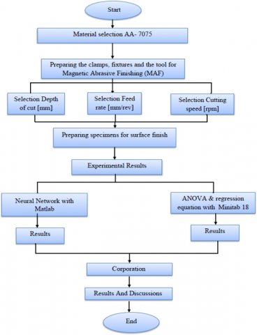
The obtained previous results had achieved the excellence of one approach either regression or artificial intelligence on the other, but in this study will demonstrate that both approaches may share the same percentage of minimizing the surface roughness. Although the artificial intelligence representing by ANN has its superiority for its modernity and simplicity. Figure 1 shown below represent the flow chat for the presented work.
Figure 1. Flow chart algorithm steps for the modelling of the surface roughness
The cutting tool CNC machine has been used to perform the experimental work. Al- 7075 was used to determine the result of the optimization process on the Al parameters. Work piece dimensions of AL was 100 × 150 × 3 mm during the milling process. The significant chemical structure of Al-7075 alloy is listed in Table 1. The value of the surface roughness was calculated with the surface roughness tester. The input parameters [speed of cut (rpm) with the feed rate (mm/rev) and the depth of cut (mm)] were used to estimate the value of the surface roughness (Ra) after machining process through performing orthogonal array L27 experiments. Since this input variables are multi-level parameters with non-linear responses. Therefore, three level tests were considered for each parameter. Table 2 demonstrates the data from experiments for the Al-7075 from orthogonal array L27.
Table 1. Chemical composition of Al-7075 alloy
|
Cr |
0.18 |
|
Fe |
0.19 |
|
Cu |
1.53 |
|
Mn |
0.07 |
|
Mg |
2.55 |
|
Ni |
0.005 |
|
Zn |
5.89 |
|
Al |
Rest |
|
Ti |
0.024 |
|
Si |
0.1 |
Table 2. The experimental data for the Al7075 from orthogonal array L27
|
NO. |
Depth of cut (mm) |
Feed rate (mm/rev) |
Cutting speed (rpm) |
Ra[µm] |
PREDICTD |
RESIDUAL |
|
1 |
0.3 |
30 |
1200 |
2.250 |
2.223 |
0.026 |
|
2 |
0.5 |
30 |
1200 |
1.370 |
1.459 |
-0.089 |
|
3 |
0.7 |
30 |
1200 |
1.050 |
0.921 |
0.128 |
|
4 |
0.3 |
50 |
1200 |
2.150 |
2.147 |
0.002 |
|
5 |
0.5 |
50 |
1200 |
1.380 |
1.437 |
-0.057 |
|
6 |
0.7 |
50 |
1200 |
0.780 |
0.952 |
-0.172 |
|
7 |
0.3 |
70 |
1200 |
2.110 |
2.145 |
-0.035 |
|
8 |
0.5 |
70 |
1200 |
1.600 |
1.487 |
0.112 |
|
9 |
0.7 |
70 |
1200 |
1.140 |
1.056 |
0.083 |
|
10 |
0.3 |
30 |
1400 |
2.250 |
2.150 |
0.099 |
|
11 |
0.5 |
30 |
1400 |
1.410 |
1.441 |
-0.031 |
|
12 |
0.7 |
30 |
1400 |
0.970 |
0.958 |
0.011 |
|
13 |
0.3 |
50 |
1400 |
2.098 |
2.134 |
-0.036 |
|
14 |
0.5 |
50 |
1400 |
1.450 |
1.464 |
-0.014 |
|
15 |
0.7 |
50 |
1400 |
1.100 |
1.020 |
0.079 |
|
16 |
0.3 |
70 |
1400 |
2.200 |
2.192 |
0.007 |
|
17 |
0.5 |
70 |
1400 |
1.560 |
1.560 |
-0.000 |
|
18 |
0.7 |
70 |
1400 |
1.040 |
1.155 |
-0.115 |
|
19 |
0.3 |
30 |
1600 |
1.980 |
2.041 |
-0.061 |
|
20 |
0.5 |
30 |
1600 |
1.350 |
1.386 |
-0.036 |
|
21 |
0.7 |
30 |
1600 |
0.910 |
0.958 |
-0.048 |
|
22 |
0.3 |
50 |
1600 |
2.160 |
2.085 |
0.075 |
|
23 |
0.5 |
50 |
1600 |
1.500 |
1.455 |
0.044 |
|
24 |
0.7 |
50 |
1600 |
1.130 |
1.051 |
0.078 |
|
25 |
0.3 |
70 |
1600 |
2.124 |
2.202 |
-0.078 |
|
26 |
0.5 |
70 |
1600 |
1.670 |
1.596 |
0.073 |
|
27 |
0.7 |
70 |
1600 |
1.170 |
1.217 |
-0.047 |
2.1 Modelling of surface roughness using design of experiments
The design of the experiment considers as a technique used to analyze and model a system response from multi input variables. Therefore, in the current study the full factorial design (FFD) has been used to study the effect of the system input parameters [speed of cut (rpm), the feed rate (mm/rev) and the depth of cut (mm)] with three levels as depicted in Table 3.
Table 3. System process parameters and their levels.
|
NO. |
Process Parameters |
1 |
2 |
3 |
|
1 |
Cutting speed [rpm] |
1200 |
1400 |
1600 |
|
2 |
Feed rate [mm/rev] |
30 |
50 |
70 |
|
3 |
Depth of cut [mm] |
0.3 |
0.5 |
0.7 |
$\begin{aligned} R_{a}=b_{0}+b_{1} * & X_{1}+b_{2} * X_{2}+b_{3} * X_{3}+b_{11} * X_{1}^{2} \\ &+b_{22} * X_{2}^{2}+b_{33} * X_{3}^{2}+b_{12} \\ & * X_{1} * X_{2}+b_{13} * X_{1} * X_{3}+b_{23} \\ & * X_{2} * X_{3}+b_{123} * X_{1} * X_{2} * X_{3} \end{aligned}$ (1)
where: Ra – represents the output surface roughness Ra (µm); X1–represent cutting speed (rpm); X2– feed rate (mm/rev); X3– depth of cut (mm). b1, b2, b3– represent regression coefficients for cutting speed (rpm), feed rate (mm/rev) and depth of cut (mm). b11, b22, b33– represent the squared coefficients of the main factors. b12, b13, b23, b123– represents the interactions among coefficients. While the b0 is a free number.
2.1.1 Regression analysis and design matrix experimental results
According to the obtained experimental data, Statistical software release 10.0 has been implemented to analyse the significance of the independent variables (factors) individually (cutting speed (rpm), feed rate (mm/rev) and depth of cut (mm). Beside their interactive coefficients as numerical values on the indicated output the surface roughness Ra (µm). Along these lines, a mathematical model relating the actual domain of independent factors with the experimental results of surface roughness has been developed using the Gauss-Newton approach through, a quadratic polynomial regression model. The fitting model results are depicted in Table 4. seeing that the main parameters with their interaction (b0, b1, b2, b3, b11, b22, b33, b12, b13, b23, b123) which illustrate the high significance with p-values.
Table 4. Regression analysis and significant coefficients according to ANOVA model
|
b0 |
5.043 |
2.523 |
0.00 |
0.00 |
-0.306 |
10.393 |
|
b1 |
-8.758 |
3.280 |
0.00 |
0.00 |
-15.71 |
-1.803 |
|
b2 |
-0.039 |
0.032 |
0.00 |
0.00 |
-0.108 |
0.030 |
|
b3 |
-0.000 |
0.002 |
0.00 |
0.00 |
-0.006 |
0.006 |
|
b11 |
2.822 |
0.975 |
0.00 |
0.00 |
0.753 |
4.890 |
|
b22 |
0.000 |
0.000 |
0.00 |
0.00 |
-0.000 |
0.000 |
|
b33 |
-0.000 |
0.000 |
0.00 |
0.00 |
-0.000 |
-0.000 |
|
b12 |
0.034 |
0.059 |
0.00 |
0.00 |
-0.091 |
0.160 |
|
b13 |
0.001 |
0.002 |
0.00 |
0.00 |
-0.002 |
0.006 |
|
b23 |
0.000 |
0.000 |
0.00 |
0.00 |
-0.000 |
0.000 |
|
b123 |
-0.000 |
0.000 |
0.00 |
0.00 |
-0.000 |
0.000 |
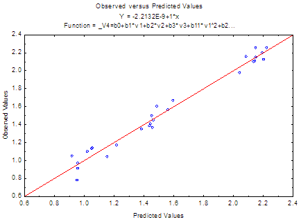
While Table 5 appropriately verified the perfection of fitness model by ANOVA results, in which the F-value of (6.439) refers to model significance. Moreover, the model fitting validity was proved in Figure 2.a&b. It is obvious that, the value of R2 = 0.987 reverse slight difference between the experimental and predicted response calculations. This indicate that the surface finishing process has been properly described by the proposed quadratic polynomial model with the process parameter that contain one dependent variable and three independent variables.
Table 5. Verified the perfection of fitness model by ANOVA results
|
Regression |
70.836 |
11.000 |
6.439 |
6.439 |
0.000 |
|
Residual |
0.146 |
16.000 |
0.009 |
0.009 |
|
|
Total |
70.982 |
27.000 |
|
|
|
|
Corrected Total |
5.953 |
26.000 |
|
|
|
|
R2 |
0.987 |
|
|
|
|
|
Regression vs. Corrected Total |
70.836 |
11.000 |
6.439 |
6.439 |
0.000 |
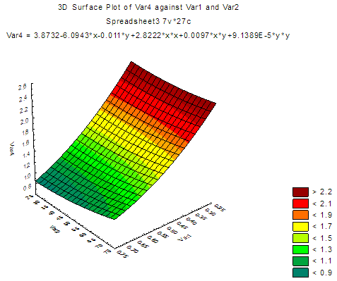
(a)
(b)
Figure 2. (a) Predicted and actual value for surface roughness; (b) Interaction of cutting speed and feed rate against surface roughness
2.2 Modelling of surface roughness using artificial neural network (ANN)
ANN has great importance due to its ability to solve the nonlinear problems [28]. Besides, ANN is used in prediction of the surface roughness in this study. ANN model with several layers was presented where the data were come from input layer and then were processed in hidden layers. Hyperbolic tangent sigmoid was the depended transfer function of the hidden layer. The hyperbolic tangent sigmoid function which is used in the proposed neural network's hidden layers, is preferred than the traditional sigmoid function because it has steady state at zero, or by other words, this function centers data in a better way for the next layer, as the output's mean is near to zero [29].
On the other hand, the hidden layer's output was fed to output layer which has the linear transfer function. The change in weights was evaluated according to Eq. (2):
$\Delta W_{j i}(n)=\alpha \Delta W_{j i}(n-1)+\eta \delta(n) Y_{i}(n)$ (2)
where, $\Delta w j(n)$ is the weights' changes: i and j =1,2,3…n; $\alpha$ represents momentum coefficient. $\delta j$ represents error; $\eta$ represents learning rate parameter and $\mathrm{Y}(n)$ represents the output at the $n t h$ iteration.
After each iteration, weights would be fed back until the minimum error percentage is obtained, which means good training of the network is achieved. Where best case takes place at regression equalling 1, at this point, the neural network will be stopped. Figure 3 shows the presented ANN model structure: Where, W: weights, and b: bias.
Figure 3. ANN model structure
Training is the first step in ANN where the inputs (cutting speed, feed rate and depth of cut) were fed to the network in addition to the surface roughness as the desired output. At first, the weights are set in random manner, which will be altered using the Back propagation algorithm to get a satisfactory performance level. Two essential methods of weights initialization exist: zero initialization and random initialization which is used in the proposed ANN model, where this technique prevents the neurons from same features learning of the inputs, this technique breaks the symmetrical results with better accuracy than zero initialization [30]. The parameters of the proposed ANN are:
3 neurons in input layer;
2 hidden layers with 10 neurons;
1 neuron in output layer;
Learning rate is 0.05;
Momentum constant is 0.95.
Weights and biases are created randomly by the MATLAB Toolbox of neural network as follows:
Weights [1,1] (to layer 1 from input 1):
$\left[\begin{array}{ccccc}0.394 & 3.307 & 1.166 ; 1.755 & 1.714 & -1.315 ; \\ -0.777 & -2.321 & 0.896 ; 2.207 & 0.092 & -2.122 ; \\ 2.811 & -0.616 & 1.627 ;-1.829 & -2.126 & -0.909 ; \\ 1.014 & -.0 .616 & 2.842:-5.297 & 0.353 & -0.362 ; \\ -2.262 & -1.385 & -1.951 ;-0.953 & -1.801 & -3.515\end{array}\right]$
Weights [2,1]: $\left[\begin{array}{rlcrr}0.431 & 0.104 & 0.413 & 0.552 & 0.562 \\ -0.357 & -0.740 & 0.634 & 0.527 & 0.293\end{array}\right]$
bias: b[1] ( bias to layer 1): $\left[\begin{array}{rrrrr}-2.681 ; & -2.435 ; & 1.894 ; & 0.0524 ; & -0.552 ; \\ 0.660 ; & 0.499 ; & 1.098 ; & -3.399 ; & 1.625\end{array}\right]$
bias: b[2]: [0.656]
The (MSE) Mean Square Error is calculated during the learning process using Eq. (3):
$\mathrm{MSE}=\frac{1}{2} \sum_{i=1}^{n}\left|T_{i}-Y_{i}\right|$ (3)
where $\mathrm{T}_{i}$ and $\mathrm{Y}_{i}$ are the Target and output values of surface roughness respectively. Then, weights which are between hidden and output layers are adjusted and calculated by Eq. (1). For developing the presented ANN model, the network is trained using 27 experiments. The network showed good training and learning to predict the output value of surface roughness for testing and validation.
It is obvious from Figure 4 above that during the training process most of the predicted and experimental values coincide very well on regression line which reaches to R=0.996in training values, it is found that regression is equal to 0.999 and 0.978 for validation and testing respectively, while regression was 0.987 in overall values performance which is a very good result. Generally, many reasons may lead to the existence of some actual values that are not very consistent to the predicted ones. These reasons may be caused by faults in experimental results due to environment, instruments and observations. Besides to the fact that the residuals are not being both negative and positive then the neural network model will not deliver a coincidence between predicted and actual values.
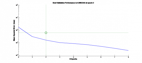
In Figure 5 above, it is clear that the performance of the presented network depended on the amount of the mean square in relation with the increment in number of epochs, where very good training was achieved, and the best validation performance was 0.006 at epoch number 2.
Table 6 shows the percentage of error of the regression models and Artificial Neural network. Each maximum error obtained in the regression models and Artificial Neural network is (0.209) and (0.287), respectively, Table 6 also shows that the regression models and Artificial Neural network minimum errors are (-0.002) and (-0.008), respectively. It can be concluded that the Artificial Neural network model produces more high accuracy results than the regression model based on the R2, MSE and errors evaluated.
Figure 4. Neural network training regression
Figure 5. ANN Mean square error
Table 6. Comparison between regression model and the neural network prediction
|
No. |
Cutting speed (rpm) |
Feed rate (mm/rev) |
Depth of cut (mm) |
Ra[µm] |
Regression |
ANN |
||
|
Output |
Error |
Out put |
Error |
|||||
|
1 |
1200 |
30 |
0.3 |
2.250 |
2.040 |
0.209 |
2.232 |
0.017 |
|
2 |
1200 |
30 |
0.5 |
1.370 |
1.483 |
-0.113 |
1.378 |
-0.008 |
|
3 |
1200 |
30 |
0.7 |
1.050 |
0.925 |
0.124 |
1.051 |
-0.001 |
|
4 |
1200 |
50 |
0.3 |
2.150 |
2.100 |
0.049 |
2.229 |
-0.079 |
|
5 |
1200 |
50 |
0.5 |
1.380 |
1.542 |
-0.162 |
1.302 |
0.077 |
|
6 |
1200 |
50 |
0.7 |
0.780 |
0.985 |
-0.205 |
0.857 |
-0.077 |
|
7 |
1200 |
70 |
0.3 |
2.110 |
2.159 |
-0.049 |
2.135 |
-0.025 |
|
8 |
1200 |
70 |
0.5 |
1.600 |
1.602 |
-0.002 |
1.590 |
0.009 |
|
9 |
1200 |
70 |
0.7 |
1.140 |
1.045 |
0.094 |
1.077 |
0.062 |
|
10 |
1400 |
30 |
0.3 |
2.250 |
2.049 |
0.200 |
1.962 |
0.287 |
|
11 |
1400 |
30 |
0.5 |
1.410 |
1.492 |
-0.082 |
1.411 |
-0.001 |
|
12 |
1400 |
30 |
0.7 |
0.970 |
0.934 |
0.035 |
0.983 |
-0.013 |
|
13 |
1400 |
50 |
0.3 |
2.098 |
2.109 |
-0.011 |
2.167 |
-0.069 |
|
14 |
1400 |
50 |
0.5 |
1.450 |
1.551 |
-0.101 |
1.437 |
0.012 |
|
15 |
1400 |
50 |
0.7 |
1.100 |
0.994 |
0.105 |
1.024 |
0.075 |
|
16 |
1400 |
70 |
0.3 |
2.200 |
2.168 |
0.031 |
2.127 |
0.072 |
|
17 |
1400 |
70 |
0.5 |
1.560 |
1.611 |
-0.051 |
1.589 |
-0.029 |
|
18 |
1400 |
70 |
0.7 |
1.040 |
1.054 |
-0.014 |
1.122 |
-0.082 |
|
19 |
1600 |
30 |
0.3 |
1.980 |
2.058 |
-0.078 |
1.958 |
0.021 |
|
20 |
1600 |
30 |
0.5 |
1.350 |
1.501 |
-0.151 |
1.443 |
-0.093 |
|
21 |
1600 |
30 |
0.7 |
0.910 |
0.944 |
-0.030 |
0.903 |
0.006 |
|
22 |
1600 |
50 |
0.3 |
2.160 |
2.118 |
0.041 |
2.157 |
0.002 |
|
23 |
1600 |
50 |
0.5 |
1.500 |
1.561 |
-0.060 |
1.470 |
0.029 |
|
24 |
1600 |
50 |
0.7 |
1.130 |
1.003 |
0.126 |
1.216 |
-0.086 |
|
25 |
1600 |
70 |
0.3 |
2.124 |
2.178 |
-0.054 |
2.191 |
-0.067 |
|
26 |
1600 |
70 |
0.5 |
1.670 |
1.620 |
0.049 |
1.654 |
0.015 |
|
27 |
1600 |
70 |
0.7 |
1.170 |
1.063 |
0.106 |
1.168 |
0.001 |
It is observed in Table 6 that:
Finally, the best value of surface roughness, according to the artificial neural network model was at 0.875 µm, when the cutting speed was1200 rpm, the feed rate was 50 mm/rev and the depth of cut was 0.7 mm, that are the same machining process parameters in which best R of experimental data took place, this is a good indication for the ANN effectiveness.
In addition, all best values of R in experimental, regression and ANN, share the property of occurring at the least speed of cutting (between the proposed ones) which is 1200 rpm. While the feed rate ranges between the least and middle values, which are either 30 and 50 mm/rev. The depth of cut was 0.7 mm in all three best values, this value was the biggest among proposed depth of cut values.
According to these data, minimum surface roughness in this milling process, was obtained at the least cutting speed, approximately middle feed rate and greater depth of cut.
In the current study, modelling and prediction for the surface roughness of 7075 Aluminium alloy were achieved using regression analysis and artificial neural network. The results of regression model estimation showed that the value of surface roughness was (0.98764 which is approximately 0.987) with an acceptable estimation for the regression equation while the value obtained from the NN was (0.98724 which is approximately 0.987). It is found that both of the models had reduced the minimum surface roughness value of the experimental data at about 0.987%. Very similar results in minimizing the surface roughness. Overall, it could be stated that the regression has given a little better result when it is compared with ANN in prediction of the minimum surface roughness.
Both of regression and artificial neural network presented promised methods to estimate the behaviour of surface roughness as a result to the changing in machining process parameters. In fact, with these reasonable results, NN can be considered as a powerful tool to estimate surface roughness value due to its easiness and ability to predicate the response of the nonlinear system. The following recommendations are suggested for future work:
1. Using another method to optimization the factors and compare them, such as the comparison between the Taguchi method and the Fuzzy Logic method
2. introducing other inputs variables such as changing the shape of the tool and obtaining other outputs such as the metal removal rate.
[1] Ali, I., Quazi, M.M., Zalnezhad, E., Sarhan, A.A., Sukiman, N.L., Ishak, M. (2019). Hard anodizing of aerospace AA7075-T6 aluminum alloy for improving surface properties. Transactions of the Indian Institute of Metals, 72(10): 2773-2781. https://doi.org/10.1007/s12666-019-01754-5
[2] Su, R.M., Qu, Y.D., Li, R.D., You, J.H. (2015). Influence of RRA treatment on the microstructure and stress corrosion cracking behavior of the spray-formed 7075 alloy. Materials Science, 51(3): 372-380. https://doi.org/10.1007/s11003-015-9851-7
[3] Verma, N., Vettivel, S.C. (2018). Characterization and experimental analysis of boron carbide and rice husk ash reinforced AA7075 aluminium alloy hybrid composite. Journal of Alloys and Compounds, 741: 981-998. https://doi.org/10.1016/j.jallcom.2018.01.185
[4] Sharma, V.K., Kumar, V., Joshi, R.S. (2020). Parametric study of aluminium-rare earth based composites with improved hydrophobicity using response surface method. Journal of Materials Research and Technology, 9(3): 4919-4932. https://doi.org/10.1016/j.jmrt.2020.03.011
[5] Palanikumar, K., Karthikeyan, R. (2006). Optimal machining conditions for turning of particulate metal matrix composites using Taguchi and response surface methodologies. Machining Science and Technology, 10(4): 417-433. https://doi.org/10.1080/10910340600996068
[6] Box, G.E., Wilson, K.B. (1992). On the experimental attainment of optimum conditions. In Breakthroughs in Statistics, pp. 270-310. https://doi.org/10.1007/978-1-4612-4380-9_23
[7] Tan, C.H., Ghazali, H.M., Kuntom, A., Tan, C.P., Ariffin, A.A. (2009). Extraction and physicochemical properties of low free fatty acid crude palm oil. Food Chemistry, 113(2): 645-650. https://doi.org/10.1016/j.foodchem.2008.07.052
[8] Khajeh, M. (2011). Response surface modelling of lead pre-concentration from food samples by miniaturised homogenous liquid–liquid solvent extraction: Box–Behnken design. Food Chemistry, 129(4): 1832-1838. https://doi.org/10.1016/j.foodchem.2011.05.123
[9] Huang, W., Li, Z., Niu, H., Li, D., Zhang, J. (2008). Optimization of operating parameters for supercritical carbon dioxide extraction of lycopene by response surface methodology. Journal of Food Engineering, 89(3): 298-302. https://doi.org/10.1016/j.jfoodeng.2008.05.006
[10] Wang, S., Jian, G., Xiao, J., Wen, J., Zhang, Z. (2017). Optimization investigation on configuration parameters of spiral-wound heat exchanger using genetic aggregation response surface and multi-objective genetic algorithm. Applied Thermal Engineering, 119: 603-609. https://doi.org/10.1016/j.applthermaleng.2017.03.100
[11] Ganguli, R., Rajagopal, S. (2009). Multidisciplinary design optimization of an UAV wing using kriging based multi-objective genetic algorithm. In 50th AIAA/ASME/ASCE/AHS/ASC Structures, Structural Dynamics, and Materials Conference, Palm Springs, California. https://doi.org/10.2514/6.2009-2219
[12] Zhu, W., Yu, X., Wang, Y. (2019). Layout optimization for blended wing body aircraft structure. International Journal of Aeronautical and Space Sciences, 20(4): 879-890. https://doi.org/10.1007/s42405-019-00172-7
[13] Mulik, R.S., Pandey, P.M. (2011). Magnetic abrasive finishing of hardened AISI 52100 steel. The International Journal of Advanced Manufacturing Technology, 55(5): 501-515. https://doi.org/10.1007/s00170-010-3102-8
[14] Shaik, J.H., Srinivas, J. (2017). Optimal selection of operating parameters in end milling of Al-6061 work materials using multi-objective approach. Mechanics of Advanced Materials and Modern Processes, 3(1): 1-11. https://doi.org/10.1186/s40759-017-0020-6
[15] Acayaba, G.M.A., de Escalona, P.M. (2015). Prediction of surface roughness in low speed turning of AISI316 austenitic stainless steel. CIRP Journal of Manufacturing Science and Technology, 11: 62-67. https://doi.org/10.1016/j.cirpj.2015.08.004
[16] Kumar, J.P., Thirumurugan, K. (2012). Optimization of machining parameters for milling titanium using Taguchi method. Int. J. Adv. Eng. Technol, 3(2): 108-113.
[17] Patel, G.M., Lokare, D., Chate, G.R., Parappagoudar, M. B., Nikhil, R., Gupta, K. (2020). Analysis and optimization of surface quality while machining high strength aluminium alloy. Measurement, 152: 107337. https://doi.org/10.1016/j.measurement.2019.107337
[18] Das, P., Mukherjee, S., Ganguly, S., Bhattacharyay, B. K., Datta, S. (2009). Genetic algorithm based optimization for multi-physical properties of HSLA steel through hybridization of neural network and desirability function. Computational Materials Science, 45(1): 104-110. https://doi.org/10.1016/j.commatsci.2008.03.050
[19] Zerti, A., Yallese, M.A., Zerti, O., Nouioua, M., Khettabi, R. (2019). Prediction of machining performance using RSM and ANN models in hard turning of martensitic stainless steel AISI 420. Proceedings of the Institution of Mechanical Engineers, Part C: Journal of Mechanical Engineering Science, 233(13): 4439-4462. https://doi.org/10.1177/0954406218820557
[20] Das, B., Roy, S., Rai, R.N., Saha, S.C. (2015). Studies on effect of cutting parameters on surface roughness of al-cu-TiC MMCs: an artificial neural network approach. Procedia Computer Science, 45: 745-752. https://doi.org/10.1016/j.procs.2015.03.145
[21] Nain, S.S., Sihag, P., Luthra, S. (2018). Performance evaluation of fuzzy-logic and BP-ANN methods for WEDM of aeronautics super alloy. MethodsX, 5: 890-908. https://doi.org/10.1016/j.mex.2018.04.006
[22] Unune, D.R., Nirala, C.K., Mali, H.S. (2018). ANN-NSGA-II dual approach for modeling and optimization in abrasive mixed electro discharge diamond grinding of Monel K-500. Engineering Science and Technology, an International Journal, 21(3): 322-329. https://doi.org/10.1016/j.jestch.2018.04.014
[23] Conde, A., Arriandiaga, A., Sanchez, J.A., Portillo, E., Plaza, S., Cabanes, I. (2018). High-accuracy wire electrical discharge machining using artificial neural networks and optimization techniques. Robotics and Computer-Integrated Manufacturing, 49: 24-38. https://doi.org/10.1016/j.rcim.2017.05.010
[24] Singh, B., Misra, J.P. (2019). Surface finish analysis of wire electric discharge machined specimens by RSM and ANN modeling. Measurement, 137: 225-237. https://doi.org/10.1016/j.measurement.2019.01.044
[25] Krishnamoorthy, A., Boopathy, S.R., Palanikumar, K. (2011). Delamination prediction in drilling of CFRP composites using artificial neural network. Journal of Engineering Science and Technology, 6(2): 191-203.
[26] Markopoulos, A.P., Georgiopoulos, S., Kinigalakis, M., Manolakos, D.E. (2016). Adaptive neuro-fuzzy inference system for end milling. Journal of Engineering Science and Technology, 11(9): 1234-1248.
[27] Bikku, T., SREE, K.S. (2020). Deep learning approaches for classifying data: A review. Journal of Engineering Science and Technology, 15(4): 2580-2594.
[28] Rajeev, D., Dinakaran, D., Kanthavelkumaran, N., Austin, N. (2018). Predictions of tool wear in hard turning of AISI4140 steel through artificial neural network, fuzzy logic and regression models. International Journal of Engineering, 31(1): 32-37. https://doi.org/10.5829/ije.2018.31.01a.05
[29] Witten, I.H., Frank, E., Hall, M.A., Pal, C.J., DATA, M. (2005). Practical machine learning tools and techniques. In Data Mining. https://faculty.kutztown.edu/parson/spring2021/WekaChapter12.pdf.
[30] Patel, P., Nandu, M., Raut, P. (2018). Initialization of weights in neural networks. International Journal of Scientific Development and Research, 3(11): 73-79.