Abdul-Nasser Nofal* | Abdel-Nasser Assimi | Yasser M. Jaamour
© 2021 IIETA. This article is published by IIETA and is licensed under the CC BY 4.0 license (http://creativecommons.org/licenses/by/4.0/).
OPEN ACCESS
In this paper, we propose two algorithms for joint power allocation and bit-loading in multicarrier systems using discrete modulations. The objective is to maximize the data rate under the constraint of a suitable Bit Error Rate per subcarrier. The first algorithm is based on the Lagrangian Relaxation of the discrete optimization problem in order to find an initial solution. A discrete solution is found by bit truncation followed by an iterative modulation adjustment. The second algorithm is based on Discrete Coordinate Ascent framework with iterative modulation increment of one selected subcarrier at each iteration. A simple cost function related to the power increment per bit is used for subcarrier selection. A sub-optimal low complexity Discrete Coordinate Ascent algorithm is proposed that overcome the limitations of the Hughes-Hartogs algorithm. The Lagrangian Relaxation algorithm provides a suboptimal solution for non-coded system using M-QAM modulations, whereas the low complexity Discrete Coordinate Ascent algorithm provides a near optimal solution for coded as well as for non-coded system using an arbitrary modulation set. Numerical results show the efficiency of the proposed algorithms in comparison with traditional methods.
adaptive modulation, bit-loading, data rate maximization, discrete modulation, Hughes-Hartogs algorithm, multicarrier system, power allocation
Emerging wireless systems increasingly require high data rates for various applications. This challenge faces multiple obstacles such as limited channel bandwidth and limited transmission power. Different Quality of Service (QoS) is required depending on the application. For example, voice and video communications tolerate errors more than file transfer [1]. Hence, the need for an efficient transmission system with a high spectral efficiency and controllable QoS is justified. Multicarrier system is widely adopted in many standards [2, 3], such as OFDM due to its robustness against channel fading and its flexible resource allocation.
The problem of maximizing data rate and minimizing transmission power is widely investigated in the literature. Since the objective of data rate maximization is controversial with the objective of total transmission power minimization, research papers followed three directions. The first direction focuses on margin maximization where the primary objective is to reduce the total transmitted power for a given data rate. An adaptive power loading algorithm with uniform bit allocation is proposed for constant data rate [4]. Other works [5, 6] proposed bit-loading algorithm with a fixed rate is proposed based on the Gap Approximation [7].
The second direction focuses on rate maximization under a fixed power constraint. Water-Filling (WF) power-allocation solution [8] is the famous example for this direction where the channel capacity is maximized. Adaptive Modulation and Coding (AMC) schemes are used to exploit the channel capacity in order to increase the data rate for a given bit error rate (BER) requirements. An incremental bit loading algorithm is proposed to maximize the data rate under a target mean BER constraint [9]. However, uniform power allocation for all subcarriers is assumed. Hughes-Hartogs (HH) [10] proposed an iterative algorithm which is referred herein as the HH algorithm. In HH algorithm, the modulation order is incremented for the subcarrier that minimize the marginal incremental power per bit at each iteration until the total power is exhausted. It is asymptotically optimal for large number of subcarriers. However, it cannot be applied for an arbitrary set of modulations. A low complexity variant of the HH algorithm is proposed for a constant BER threshold for all subcarriers [11].
The third direction focuses on finding a trade-off between high data rate and low total transmitted power. The multi-objective optimization problem is transformed by linear combination between bitrate and power objectives. Different solution can be found for different linear coefficients. Works are examples for this type of optimization. In general, this approach suffers from scaling problem between different objective functions [12, 13]. Therefore, there is no clear quantitative measure on how to choose the linear combination coefficients. In addition, convergence problems can be encountered for extreme values of these coefficients.
This paper follows the second direction where the primary goal is to achieve the maximum possible data rate. In practical systems, the absolute achievable data rate is limited by the highest modulation order supported by the system. When the absolute data rate is achieved in good channel conditions, the first direction is taken by minimizing the transmission power as a secondary objective. The main contribution in this paper is the proposal of two algorithms for discrete joint power allocation and bit-loading with comprehensive derivation. The first algorithm presents a comprehensive method with water-filling analogy for non-coded systems using an arbitrary M-QAM modulation set. The second algorithm is a generalization of the HH algorithm for coded and non-coded systems with an arbitrary modulation set. By pointing to the limitation of the HH algorithm for some constellation sets, we propose a heuristic cost function that overcomes this limitation.
The rest of the paper is organized as follows: In Section 2, the adopted system model is introduced. Then the formulation of the discrete optimization problem is given in Section 3. The two proposed algorithms are then described in Section 4 and Section 5 respectively. After that, a low complexity discrete algorithm is proposed in section 5. Finally, numerical results are shown in section 7.
The considered system is a multicarrier system with N independent parallel fading channels. For each subcarrier $i=$ $1,2, \ldots, N$, the transmitter modulates $b_{i}$ bits into a complex symbol $s_{i}$ taken from a constellation $C_{k}$ having $2^{b_{i}}$ symbols and unit average power. $C_{k}$ is selected from a set of complex constellations $\left\{C_{k}: k=0,1, \ldots, K\right\}$ according to an adopted bit-loading strategy. The size of $C_{k}$ is $2^{m_{k}}$ symbols which can carry $m_{k}$ bits. In this paper, we assume that the constellation $C_{0}$ is always included in the set and corresponds to the null constellation with $m_{0}=0 .$ In addition, we assume that the constellation set is ordered in the increasing order of the number of carried bits with $m_{0}<m_{1}<\cdots<m_{K}$. For example, a possible choice for the constellation set can be $\left\{C_{0}: N u l l, C_{1}: 4-\mathrm{QAM}, C_{2}: 16-\mathrm{QAM}, C_{3}: 64-\mathrm{QAM}\right\}$. In this example, the number of modulated bits $b_{i}$ takes one of the following values: $\left\{m_{0}=0, m_{1}=2, m_{2}=4, m_{3}=6\right\}$. The index $k$ of the selected constellation is called herein the modulation index. The modulated symbol $s_{i}$ is multiplied by a power factor $\sqrt{p_{i}}$ before being transmitted over subcarrier $\mathrm{i}$.
The received signal $r_{i}$ on subcarrier i is modeled as
$r_{i}=g_{i} \sqrt{p_{i}} s_{i}+w_{i} ; i=1, \ldots, N$, (1)
where, $g_{i}$ is the complex channel gain, and $w_{i}$ is an Additive White Gaussian Noise (AWGN) with power of $\sigma_{n}^{2}$. The received signal to noise ratio $S N R_{i}$ on subcarrier i is given by
$\mathrm{SNR}_{i}=p_{i} \frac{\left|g_{i}\right|^{2}}{\sigma_{n}^{2}}=p_{i} \gamma_{i}$ (2)
where, $\gamma_{i} \equiv\left|g_{i}\right|^{2} / \sigma_{n}^{2}$.
The objective in this paper is to maximize total data throughput in a multicarrier system using a discrete modulation set with a limited total power budget $P_{\max }$ under the constraint of a given QoS per subcarrier. In other words, the objective is to maximize the spectral efficiency in the system by sending the maximum number of bits per transmission with the lowest possible power that guarantees the required QoS. The QoS constraint is expressed by a given bit error rate threshold $\mathrm{BER}_{i, t h}$ per subcarrier.
The optimization problem can be formulated as
$\underset{b_{i}, p_{i}}{\operatorname{Maximize}} B_{T} \equiv \sum_{i=1}^{N} b_{i}$ (3)
Subject to
$\begin{aligned}
&\mathrm{BER}_{i} \leq \mathrm{BER}_{t h, i}, i=1, \ldots, N, \\
&P_{T} \equiv \sum_{i=1}^{N} p_{i} \leq P_{\max }\quad ; \\
&p_{i} \geq 0 ; i=1, \ldots, N ; \\
&b_{i} \in \mathcal{M}=\left\{m_{0}, m_{1}, \ldots, m_{K}\right\}\quad;
\end{aligned}$
where, $\mathrm{BER}_{i}$ is the BER for subcarrier $\mathrm{i}$, and $\mathcal{M}$ is the set of possible transmitted bits per symbol. This is a discrete optimization problem with inequality constraints. A possible approach to solve this problem is to relax the last constraint in (3) related to $b_{i}$ values by allowing $b_{i}$ to take real positive values in order to use Lagrange multipliers method to find an initial solution [13]. The initial founded solution for $b_{i}$ by Lagrangian relaxation (LR) is then rounded to nearest integers with additional heuristic readjustments steps which are applied on the optimization variables $b_{i}$ and $p_{i}$. This is the adopted approach for the first proposed algorithm in the next section, we propose a near optimal, yet simple algorithm that removes all the previous disadvantages of the LR approach.
3.1 Lagrangian relaxation
Relaxing the last constraint in (3) on the number of loaded bits by allowing $b_{i}$ to take real values, this constraint becomes
$0 \leq b_{i} \leq b_{i, \max }$ (4)
where, $b_{i, \max }$ is the maximum allowable loaded bits on carrier i.
For M-QAM modulation, BER for subcarrier i can be approximated as in [4],
$\operatorname{BER}_{i}\left(b_{i}, p_{i}, \gamma_{i}\right) \approx 0.2 \exp \left(-\frac{1.6 p_{i} \gamma_{i}}{2^{b_{i}}-1}\right)$ (5)
This approximation is tight within 1 dB for $\mathrm{BER} \leq 10^{-3}$. The required power to achieve the target bit error rate $\mathrm{BER}_{i, t h}$ must be greater than a specific threshold [13, 14]
$p_{i} \geq-\ln \left(5 \times \mathrm{BER}_{i, t h}\right) \frac{2^{b_{i}}-1}{1.6 \gamma_{i}}=P_{t h, i}$ (6)
$P_{t h, i} \equiv\left(2^{b_{i}}-1\right) \frac{\alpha_{i}}{\gamma_{i}}$ (7)
where, $\alpha$ is defined as $\alpha_{i} \equiv-\ln \left(5 \times \mathrm{BER}_{i, t h}\right) / 1.6$.
In addition, the BER constraint can be replaced with the following constraint
$P_{t h, i}-p_{i} \leq 0$ (8)
The new optimization problem can be formulated as
$\underset{b_{i}, p_{i}}{\text { Maximize }} B_{T} \equiv \sum_{i=1}^{N} b_{i}$ (9)
Subject to
$\begin{aligned}
&P_{t h, i}-p_{i} \leq 0 ; i=1, \ldots, N; \\
&P_{T} \equiv \sum_{i=1}^{N} p_{i} \leq P_{\max }\quad; \\
&p_{i} \geq 0 ; \quad i=1, \ldots, N ; \\
&0 \leq b_{i} \leq b_{i, \max } ; i=1, \ldots, N\quad;
\end{aligned} $
The objective function in (9) is a convex and the problem can be solved using Lagrange multipliers method. By transforming inequality constraints in (9) into equality constraints by using slack variables, the Lagrange function can be expressed as
$\begin{aligned}
&\mathcal{L}(\mathbf{b}, \mathbf{p}, \lambda, \boldsymbol{\Theta}, \boldsymbol{\Omega}, x, \boldsymbol{y}, \mathbf{z}) \\
&\qquad \begin{aligned}
&=\sum_{i=1}^{N} b_{i} \\
&-\lambda\left(\sum_{i=1}^{N} p_{i}-P_{\max }+x^{2}\right) \\
&-\sum_{i=1}^{N} \theta_{i}\left(\left(2^{b_{i}}-1\right) \frac{\alpha_{i}}{\gamma_{i}}-p_{i}+y_{i}^{2}\right) \\
&-\sum_{i=1}^{N} \omega_{i}\left(b_{i}-b_{i, \max }+z_{i}^{2}\right)
\end{aligned}
\end{aligned}$ (10)
where, $\quad \mathbf{b}=\left[b_{1}, \ldots, b_{N}\right]^{T}, \quad \mathbf{p}=\left[p_{1}, \ldots, p_{N}\right]^{T}$ are the optimization variables, $\lambda$ is a constant, $\boldsymbol{\Theta}=\left[\theta_{1}, \ldots, \theta_{N}\right]^{T}, \Omega=$ $\left[\Omega_{1}, \ldots, \Omega_{N}\right]^{T}$ are the multipliers variables, $x$ represents the non-used power, $\boldsymbol{y}=\left[y_{1}, \ldots, y_{N}\right]^{T}, \boldsymbol{z}=\left[z_{1}, \ldots, z_{N}\right]^{T}$ are the slack variables which are squared to ensure non-negative slack values.
A stationary point can be found by solving
$\nabla \mathcal{L}(\mathbf{b}, \mathbf{p}, \lambda, \boldsymbol{\Theta}, \boldsymbol{\Omega}, x, \boldsymbol{y}, \mathbf{z})=0$ (11)
which leads to the following equations
$\frac{\partial \mathcal{L}}{\partial b_{i}}=1-\Omega_{i}-\ln (2) \theta_{i} \frac{\alpha_{i}}{\gamma_{i}} 2^{b_{i}}=0$ (12a)
$\frac{\partial \mathcal{L}}{\partial p_{i}}=-\lambda+\theta_{i}=0$ (12b)
$\frac{\partial \mathcal{L}}{\partial \lambda}=-\left(\sum_{i=1}^{N} p_{i}-P_{\max }+x^{2}\right)=0$ (12c)
$\frac{\partial \mathcal{L}}{\partial \theta_{i}}=-\left(P_{t h, i}-p_{i}+y_{i}^{2}\right)=0$ (12d)
$\frac{\partial \mathcal{L}}{\partial \Omega_{i}}=-\left(b_{i}-b_{i, m a x}+z_{i}^{2}\right)=0$ (12e)
$\frac{\partial \mathcal{L}}{\partial x}=-2 x \lambda=0$ (12f)
$\frac{\partial \mathcal{L}}{\partial y_{i}}=-2 \theta_{i} y_{i}=0$ (12g)
$\frac{\partial \mathcal{L}}{\partial z_{i}}=-2 \Omega_{i} z_{i}=0$ (12h)
Eqns. (12a)-(12h) form 6N+2 equation with 6N+2 unknowns. The solutions of these equations can be determined by distinguishing two cases starting from resolving the Eq. (12f).
3.1.1 Case-1: Active Total Power Constraint
When $\lambda>0 \text { and } x=0$, the total power constraint is called active or binding constraint. This corresponds to the allocation of the whole available power $P_{\max }$. From (12b), we have $\theta_{i}=\lambda$. By substituting this value in (12a), we get
$\Omega_{i}=1-\ln (2) \lambda \frac{\alpha}{\gamma_{i}} 2^{b_{i}}$. (13)
Since $\lambda>0$, meaning that $\theta_{i}>0$, which leads from $(12 \mathrm{~g})$ to $y_{i}=0$. By substituting the value of $y_{i}$ in (12d), allocated powers become related to loaded bits after using the definition of $P_{t h, i}$ in (7) by
$p_{i}=P_{t h, i}=\left(2^{b_{i}}-1\right) \frac{\alpha_{i}}{\gamma_{i}}$ (14)
For convenience, and to simplify notations in the remaining analysis, a new variable η is defined as
$\eta \equiv \frac{1}{\ln (2) \lambda}$ (15)
From (12h), two subcases are discussed depending on the values of $\Omega_{i}$.When $\Omega_{i}=0$ and $z_{i}>0$, i.e subcarrier $\mathrm{i}$ is not maximally loaded $\left(b_{i}<b_{i, \max }\right)$, the solution of the optimization problem can be deduced from (14) and (16) as
$b_{i}^{*}=\log _{2}\left(\eta \times \frac{\gamma_{i}}{\alpha_{i}}\right)$ (16)
$p_{i}^{*}=\eta-\frac{\alpha_{i}}{\gamma_{i}}$ (17)
where, $\eta \equiv \frac{1}{\ln (2) \lambda}$. This a valid solution if $0 \leq b_{i}<b_{i, \max }$, which gives the following validity interval on the values of $\frac{\alpha_{i}}{\gamma_{i}}$.
$\frac{\eta}{2^{b_{i, m a x}}}<\frac{\alpha_{i}}{\gamma_{i}} \leq \eta$ (18)
When $\Omega_{i} \geq 0$ and $z_{i}=0$, i.e the subcarrier $\mathrm{i}$ is maximally loaded $\left(b_{i}=b_{i, \max }\right)$, the corresponding power allocation is given by (14), Thus the optimal solution in this case is given by
$b_{i}^{*}=b_{i, \max }$ (19)
$p_{i}^{*}=\left(2^{b_{i, m a x}}-1\right) \frac{\alpha_{i}}{\gamma_{i}}$ (20)
Which is valid for
$\frac{\alpha_{i}}{\gamma_{i}} \leq \frac{\eta}{2^{b_{i, m a x}}}$ (21)
Finally, by reassembling the previous results, the optimal solution in the case of active power constraint is given for each subcarrier as follows
$b_{i}^{*}=0$ (22)
$p_{i}^{*}=0$ (23)
$b_{i}^{*}=\log _{2}\left(\eta \times \frac{\gamma_{i}}{\alpha_{i}}\right)$ (24)
$p_{i}^{*}=\eta-\frac{\alpha_{i}}{\gamma_{i}}$ (25)
For $\frac{\alpha_{i}}{\gamma_{i}} \leq \frac{\eta}{2^{b_{i, m a x}}}$ (fully loaded subcarriers)
$b_{i}^{*}=b_{i, \max }$ (26)
$p_{i}^{*}=\left(2^{b_{i, m a x}}-1\right) \frac{\alpha_{i}}{\gamma_{i}}$ (27)
As it will be seen in the next subsection, the parameters $\eta$ represents a threshold value, which can be calculated from the active power constraint using an iterative algorithm.
3.1.2 Case-2: Inactive Total Power Constraint
This is the case when $\lambda=0$ and $x \geq 0$. This means that the used power is less than $P_{\max }$. From (12b) we have $\theta_{i}=0$ for all subcarriers. By substituting $\theta_{i}$ in (12a), we get $\Omega_{i}=1$. Again, by substituting $\Omega_{i}$ in (12h), we get $z_{i}=0$, meaning that all subcarriers are maximally loaded and a power margin $x^{2}$ is available. In this case, we have an infinity number of solutions with different values for slack variables $x$ and $y_{i}$. The solution with the minimum total power is the same as given by $(24)$ and (25).
For applications with a constant total power, the remaining power margin can be distributed on subcarriers in order to reduce BER on some selected subcarriers or to enhance the SNR on all subcarriers by the same factor. In the former, the power allocation per subcarrier can be increased by a specific ratio $\varepsilon$
$p_{i}=P_{t h, i}+\varepsilon P_{t h, i}$ (28)
The value of ε can be determined in order to have a total allocated power equal to $P_{\max }$ by
$\varepsilon=\frac{P_{\max }-\sum_{i=1}^{N} P_{t h, i}}{\sum_{i=1}^{N} P_{t h, i}}$. (29)
It can be easily verified that the total power is $P_{\max }$, and the SNR enhancement factor is ($(1+\varepsilon)$), However this does not guarantee equal BER over all subcarriers. A more sophisticated solution can be established for this purpose, but this is out the scope of this paper.
3.2 Analogy with water-filling principle
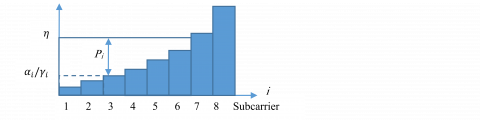
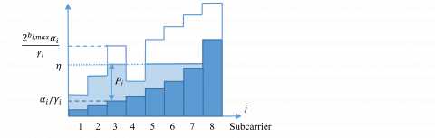
The obtained results are similar to the water filling algorithm with an additional constraint on maximum bit load. Figure 1 illustrates the water filling principle with unbounded bit load where subcarriers are reordered in the increasing value of $\alpha_{i} / \gamma_{i}$. Figure 2 shows the water-filling principle with an arbitrary bounded bit load for each subcarrier. Bounding the bit load on a subcarrier, and consequently the allocated power, will increase the threshold level in comparison with the unbounded case. The increased threshold results in an increased power allocation for other subcarriers. This may result in loading new subcarriers, which are not loaded in the unbounded case as it can be seen for subcarrier 7 on the same figure.
Figure 1. Water-Filling with unbounded bit load
Figure 2. Water-Filling with bounded bit load
3.3 Threshold value $\eta$
As mentioned before, the threshold value can be calculated from the total power constraint
$\sum_{i=1}^{N} p_{i}=P_{\max }$ (30)
Let $\mathcal{S}_{1}$ the set of subcarriers with $b_{i}=b_{i, \max }$, and let $\mathcal{S}_{2}$ the set of subcarriers with $0<b_{i}<b_{i, \max }$. The total power constraint can be rewritten as
$\sum_{i \in \mathcal{S}_{1}}\left(2^{b_{i, m a x}}-1\right) \frac{\alpha_{i}}{\gamma_{i}}+$$\sum_{i \in \mathcal{S}_{2}}\left(\eta-\frac{\alpha_{i}}{\gamma_{i}}\right)=P_{\max }$ (31)
From (30), the threshold $\eta$ is given by
$\eta=\frac{1}{N_{2}}$$\left(P_{\max }-\sum_{i \in \mathcal{S}_{1}}\left(2^{b_{i, \max }}-1\right) \frac{\alpha_{i}}{\gamma_{i}}+\sum_{i \in \mathcal{S}_{2}} \frac{\alpha}{\gamma_{i}}\right)$ (32)
where, $N_{2} \text { is the cardinality of } \mathcal{S}_{2}$
Inspired from the analogy with water filling principle presented in the previous subsection, the proposed algorithm to determine $\mathcal{S}_{1} \text { and } \mathcal{S}_{2}$ works in two scans over subcarriers. The first scan operates in the same manner as a classical water filling algorithm with unbounded bit load in order to find an initial set of loaded subcarriers. The corresponding threshold value $\eta_{1}$ is a lower bound for the final threshold. The second scan applies the bounding constraint on the bit load for each subcarrier in the increasing order of power bound. The obtained excess of power resulting from a single bounding operation is used to update the bit load and power-allocation for other remaining subcarriers. This operation continues until the upper bound is above the threshold value.
Instead of using rounding operation on real bit load to the nearest integers in the set $\mathcal{M}$, a truncation operation is performed to the lower integers in $\mathcal{M}$ and reducing the allocated power accordingly
$b_{i}^{*}=\left\lfloor\log _{2}\left(\eta \times \frac{\gamma_{i}}{\alpha_{i}}\right)\right\rfloor_{\mathcal{M}}$ (33)
$p_{i}^{*}=\left(2^{b_{i}}-1\right) \frac{\alpha_{i}}{\gamma_{i}}$ (34)
with $\lfloor \cdot\rfloor_{\mathcal{M}}$ denoting the truncation operation to the lower integer in $\mathcal{M}$. Finally, the residual power resulting from the truncation operation is used to increase the modulation index of subcarriers in an iterative manner. At each iteration, the modulation index of a selected subcarrier is increased by one. The selection criterion is based on the minimization of which is inspired from the discrete solution presented in Section 5 and given by
$C_{i}\left(k_{i}\right)=\left\{\begin{array}{cc}
P_{t h, i}\left(k_{i}+1\right), & k_{i}<k_{i, \max } \\
\infty, & k_{i}=k_{i, \max }
\end{array}\right.$ (35)
where, $P_{t h, i}\left(k_{i}+1\right)=\left(2^{m_{k_{i}}+1}-1\right) \frac{\alpha_{i}}{\gamma_{i}}$.
The iterative operation continues until the total power reaches $P_{\max }$ or all carrier are maximally loaded. The iterative algorithm will be discussed in details in Section 5. The proposed algorithm is given as follows.
|
Algorithm 1. LR algorithm |
|
|
1: |
INPUT $P_{\max }, \quad \alpha_{i} / \gamma_{i}, b_{i, \max }$ |
|
2: |
Initialize $m=N, S=\sum_{i=1}^{m} \alpha_{i} / \gamma_{i}, \mathcal{S}_{1}=\{\emptyset\}, \mathcal{S}_{2}=\{1, \ldots, N\}$ |
|
3: |
Sort $\alpha_{i} / \gamma_{i}$ in the increasing order |
|
4: |
Calculate $\eta=\left(P_{\max }+S\right) / m$ |
|
5: |
while $\alpha_{m} / \gamma_{m}>\eta$ do |
|
6: |
$S=S-\alpha_{m} / \gamma_{m}$, |
|
7: |
$\text { Remove } m \text { from } \mathcal{S}_{2}$ |
|
8: |
$m=m-1$ |
|
9: |
Update $\eta=\left(P_{\max }+S\right) / m$ |
|
10: |
end while |
|
11: |
Sort of $2^{b_{i, \max }} \alpha_{i} / \gamma_{i}$ in the increasing order and save indices in a vector $\text { I }$ |
|
12: |
Initialize $j=1, P=P_{\max }, i=\mathbf{I}(j)$ |
|
13: |
while $2^{b_{i, \max }} \alpha_{i} / \gamma_{i}<\eta$ do |
|
14: |
$P=P-\left(2^{b_{i, m a x}}-1\right) \alpha_{i} / \gamma_{i}$ |
|
15: |
$S=S-\alpha_{i} / \gamma_{i}$ |
|
16: |
$\text { Move } i \text { from } \mathcal{S}_{2} \text { to } \mathcal{S}_{1}$ |
|
17: |
$\text { Update } \eta=(P+S) /(m-j)$ |
|
18: |
$\text { while } \alpha_{m+1} / \gamma_{m+1}<\eta \text { then }$ |
|
19: |
$m=m+1$ |
|
20: |
$S=S+\alpha_{m} / \gamma_{m}$ |
|
21: |
$\text { Add } m \text { to } \mathcal{S}_{2}$ |
|
22: |
$\text { Update } \eta=(P+S) /(m-j)$ |
|
23: |
end while |
|
24: |
$j=j+1$ |
|
25: |
$i=\mathbf{I}(j)$ |
|
26: |
end while |
|
27: |
For $\mathcal{S}_{1} \text { calculate } b_{i}^{*}, \quad p_{i}^{*}$ from (23) and (24) respectively. |
|
28: |
For $\mathcal{S}_{2} \text { calculate } b_{i}^{*}, p_{i}^{*}$ from (20) and (21) respectively. |
|
29 |
Increment iteratively modulation indices in $\mathcal{S}_{2}$ using the cost function (35) until $P_{\max }$ or all carrier are maximally loaded |
|
30: |
OUTPUT $b_{i}^{*}, p_{i}^{*}$ |
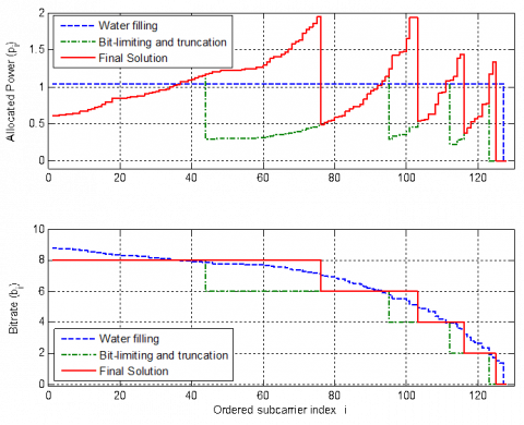
Figure 3. Power-allocation and bit-loading at different stages in the LR algorithm
Figure 3 shows and example of the obtained power allocation and bit-loading at each stage of the LR algorithm for N=128 subcarriers. The complexity of the LR algorithm without the last adjustment performed after bit truncation is $\mathcal{O}(N \log (N))$ [14], due to the sorting operation in steps 3 and 11. The complexity of the last adjustment operation will be analyzed in the next Section.
The LR approach leads in general to a suboptimal solution and has some disadvantages:
A unified closed form expression for $\mathrm{BER}_{i}$ (for all possible modulation schemes) is required to solve the problem. Resorting to some approximations is required in order to simplify the analytical derivation. Thus, it is limited to non-coded systems.
The rounding operation does not necessarily lead to an optimal discrete solution. The situation becomes worse when not using a greedy modulation set, i.e. the difference of loaded bits between two consecutive modulations is more than one bit.
In the next section, a direct discrete solution using linear programming for the optimization problem (3) is presented. The proposed solution overcomes the previous limitations of the Langrangian approach with a comparable complexity.
The principle of the discrete algorithm is to sequentially distribute bits on subcarriers with the lowest possible consumed power per bit until the total power threshold $P_{\max }$ is reached or all carriers are maximally loaded. A power cost is associated with each transmitted bit. If transmitted bits are allocated in the increasing power cost, the obtained solution is asymptotically optimal for a large number of subcarriers. Starting from the null state where no subcarrier is loaded, the allocation is performed by gradually increasing the modulation index of subcarriers in a specific order as shown by the following analysis.
For a given subcarrier i with modulation index $k_{i} \in\{1, \ldots, K\}$, the BER performance is function of received SNR, i.e.
$B E R_{i}=f_{k_{i}}\left(S N R_{i}\right)$, (36)
where, $f_{k_{i}}$ is usually a waterfall shaped monotonically decreasing function, which depends on the selected constellation $C_{k_{i}}$. The SNR threshold to achieve the target $\mathrm{BER}_{i, t h}$ is given by
$S N R_{t h, i}\left(k_{i}\right)=f_{k_{i}}^{-1}\left(B E R_{t h, i}\right)$ (37)
From (33) and (2), the minimum required power to achieve (with equality) the target $\mathrm{BER}_{i, t h}$ for a given modulation index $k_{i}$ is
$p_{i}\left(k_{i}\right)=P_{t h, i}\left(k_{i}\right)=S N R_{t h, i}\left(k_{i}\right) / \gamma_{i}$ (38)
with the assumption $P_{t h, i}(0)=\mathrm{SNR}_{t h, i}(0)=0$ for the null modulation $\left(k_{i}=0\right)$, i.e. when a subcarrier is not loaded. When increasing modulation index of a subcarrier i by one, the number of loaded bits increase by
$\Delta b_{i}\left(k_{i}\right)=m_{k_{i}+1}-m_{k_{i}}, k_{i}<k_{i, \max }$ (39)
In order to keep the BER at the target level, the allocated power is increased by
$\Delta p_{i}\left(k_{i}\right)=P_{t h, i}\left(k_{i}+1\right)-P_{t h, i}\left(k_{i}\right), k_{i}<k_{i, \max }$ (40)
The cost in term of power for each of the additional $\Delta b_{i}$ bits is then
$C_{i}\left(k_{i}\right)=\left\{\begin{array}{cc}
\frac{\Delta p_{i}\left(k_{i}\right)}{\Delta b_{i}\left(k_{i}\right)}, & k_{i}<k_{i, \max } \\
\infty, & k_{i}=k_{i, \max }
\end{array}\right.$ (41)
where,
$\frac{\Delta p_{i}\left(k_{i}\right)}{\Delta b_{i}\left(k_{i}\right)}=\frac{1}{\gamma_{i}} \frac{\mathrm{SNR}_{t h, i}\left(k_{i}+1\right)-\mathrm{SNR}_{t h, i}\left(k_{i}\right)}{m_{k_{i}+1}-m_{k_{i}}}$
Minimizing the cost function means the maximization of data rate profit per power unit. Let $\mathbf{k}=\left[k_{1}, k_{2}, \ldots, k_{N}\right]^{T} \in$ $\{0,1, \ldots, \mathrm{K}\}^{N}$ be the modulation indices for all subcarriers. The optimization problem (3) can be rewritten as an optimization problem with respect to the vector $\mathbf{k}$ as
$\underset{k_{i}}{\operatorname{Maximize}}\left(B_{T}=\sum_{i=1}^{N} m_{k_{i}}\right)$ (42)
Subject to
$\begin{aligned}
&\sum_{i=1}^{N} P_{t h, i}\left(k_{i}\right) \leq P_{\max } \\
&k_{i} \leq k_{i, \max }
\end{aligned}$
This is a discrete linear programming problem. In linear programming, it is well known that the optimum value of a concave (or convex) function is always attained on the boundary of the constraint set [15].
The proposed approach to solve this problem is based on the Coordinate Ascent (CA) framework where only one selected coordinate is stepped toward the optimum. The stepping strategy is performed by line search method where the maximization function is always increased at each iteration t, i.e. $B_{T}^{(t)}>B_{T}^{(t-1)}$.
Initially, all subcarriers are not loaded. At each subsequent iteration, the modulation index for a selected subcarrier is increased by one. The criterion for coordinate (subcarrier) selection is based on cost minimization. The selected subcarrier is given by
$i=\underset{1 \leq j \leq N}{\arg \min } \mathrm{C}_{j}\left(k_{j}\right)$ (43)
Iterations continue until reaching the stopping condition defined by the power constraint or the maximum bit-load. This procedure allows for continuously increasing the bitrate in the feasible set while being away from borders as far as possible. The corresponding algorithm is given as follows
|
Algorithm 2. Discrete Coordinate Ascent (DCA) algorithm |
|
|
1: |
INPUT $P_{\max }, \gamma_{i}, k_{i, \max }, \operatorname{BER}_{t h, i}, \mathcal{M}$ |
|
2: |
initialize $k_{i}=0, p_{i}=0$, $\text { Calculate } C_{i}, i=0, \ldots, N \text { using (41) }$ |
|
3: |
repeat |
|
4: |
Select coordinate $i$ according to (43) |
|
5: |
if $P_{T}+\Delta p_{i}\left(k_{i}\right) \leq P_{\max }$ then |
|
6: |
$P_{T}=P_{T}+\Delta p_{i}\left(k_{i}\right)$ |
|
7: |
$k_{i}=k_{i}+1$ |
|
8: |
Update $C_{i}$ using (41) |
|
9: |
end if |
|
10: |
until $P_{\max }$ is reached or all subcarriers are maximally loaded2 |
|
11: |
Calculate $p_{i}\left(k_{i}\right)$ using (38) |
|
12: |
OUTPUT $k_{i}, p_{i}$ |
The advantage of the Discrete Coordinate Ascent (DCA) in comparison with the LR that only SNR thresholds at the desired BER values are needed. This allows the use of DCA algorithm for coded systems as well as for non-codes systems. In addition, no approximation or rounding is performed. It is asymptotically optimal for large number of subcarriers. Suboptimality may occur only in the last few iterations just before reaching $P_{\max } .$ For example, if in the last iteration, there is a subcarrier $j$ other than the select subcarrier $i$ with $\Delta b_{j}\left(k_{j}\right)>$ $\Delta b_{i}\left(k_{i}\right)$ such that $P_{T}+\Delta p_{j}\left(k_{j}\right) \leq P_{\max }$, the selection of the subcarrier j leads to a better data rate while satisfying the power constraint. In other words, the subcarrier j fills the remaining power gap to $P_{\max }$ without being the more efficient in term profit. However, this has a minor effect on the overall throughput performance.
It is worth to note that the cost function given in (41) is the same cost function proposed in [10]. Consequently, the DCA algorithm leads to same solution as in HH algorithm. The previous derivation presents a comprehensive analysis for the HH method, which was proposed for a specific set of M-QAM modulations. In Section 6, we generalize the HH algorithm for an arbitrary modulation set by mean of a modified cost function.
In the DCA algorithm, the maximum number of iterations is $K N$. The complexity in each iteration is $\mathcal{O}(N)$ due to step 4 that searches for the best stepped subcarrier. Thus, the overall complexity of DCA is $\mathcal{O}\left(K N^{2}\right)$.
A low complexity variant of the DCA algorithm can be implemented when the cost function $C_{i}\left(k_{i}\right)$ for a given subcarriers is an increasing function with $k_{i}=0, \ldots, K$. Instead of searching for subcarrier that minimizes the cost function at each iteration, all values of $C_{i}\left(k_{i}\right)$ for $i=0, \ldots, N$ and $k_{i}=0, \ldots, K-1$ are pre-calculated and sorted in the increasing order. The corresponding indices $\left(i, k_{i}\right)$ are saved.
The strict monotonicity per subcarrier guarantees that the modulation index is sequentially increased by one for each subcarrier so that $\left(i, k_{i}\right)$ precedes $\left(i, k_{i}+1\right)$ after ordering. This is necessary because the cost function in (43) is defined for a single increment. Thus, the sequence of subcarrier indices at subsequent iterations in the DCA algorithm becomes identical to the sequence of subcarrier indices of the ordered values of the cost function. Using this alternative for subcarrier selection, the complexity of the DCA algorithm reduces to $\mathcal{O}(K N \log (N))[14]$ which is the complexity of the ordering operation of $\mathrm{N}$ vectors each contains $\mathrm{K}$ ordered values. This is the main idea in the HH algorithm and there are some works that confuse it with the DCA algorithm when speaking about its complexity [16,17].
The HH algorithm in [10] is proposed for the M-QAM modulation set with $\mathcal{M}_{1}=\{0,2,4,5,6,8\}$. The cost function is calculated based on the asymptotic BER performance (free distance between the constellation points). For unit free distance, the average power of M-QAM constellations is $P_{Q A M}=\{2,6,10,20,42,82,170\}$ for $\mathcal{M}=$ $\{2,3,4,5,6,7,8\}$. This leads for $\mathcal{M}_{1}$ to $C_{i}=$ $P_{t h, i}(2)\{0.5,2,5,11,32\}$ which is monotone with the modulation index. However, adding the 8 -QAM modulation in $\mathcal{M}_{1}$ results in a violation the strict monotonicity property of the cost function which becomes $\mathrm{C}_{i}=$ $P_{t h, i}(2)\{0.5,2,2,5,11,32\}$. In addition, the proposed set does not verify the monotonicity property for precise SNR threshold values.
Table 1 gives the values of $\mathrm{SNR}_{t h}$ obtained by simulation for various M-QAM modulations using Gray mapping at different levels of $\mathrm{BER}_{t h} .$ The SNR thresholds for a coded system using the convolutional code (CC) with the generator polynomial (171,131) are also reported where Viterbi algorithm was used for decoding with hard decision. It can be easily verified that for the complete M-QAM set $\{0,2,3,4,5,6,7,8\}$ the monotonicity property does not hold for a non-coded system.
Table 1. SNRth(dB) for M-QAM modulations with Gray mapping, for non-coded and coded system using CC(171,131)
|
|
Non-coded |
CC(171,131) |
||||
|
$\mathrm{BER}_{t h} \rightarrow$ |
$10^{-3}$ |
$10^{-4}$ |
$10^{-5}$ |
$10^{-3}$ |
$10^{-4}$ |
$10^{-5}$ |
|
4-QAM |
9.8 |
11.4 |
12.6 |
4.9 |
5.9 |
6.9 |
|
8-QAM |
14.4 |
16.0 |
17.3 |
9.4 |
10.2 |
11.0 |
|
16-QAM |
16.6 |
18.3 |
19.5 |
11.1 |
12.1 |
12.8 |
|
32-QAM |
19.6 |
21.2 |
22.4 |
14.9 |
16.2 |
17.0 |
|
64-QAM |
22.6 |
24.2 |
25.5 |
16.4 |
17.6 |
18.7 |
|
128-QAM |
25.4 |
27.2 |
28.5 |
19.6 |
21.0 |
22.1 |
|
256-QAM |
28.5 |
30.3 |
31.6 |
21.2 |
22.6 |
23.6 |
The exception is the 8 -QAM modulation. For the coded case, the modulations with odd number of bits have to be excluded in order to keep the monotonicity property. As example, for BERth $=10^{-5}$, the calculated cost values are $\mathrm{C}_{i}=$ $P_{t h, i}(2)\{0.5,1.45,1.26,5.40,3.76,15.30,11.63\} \quad$. By conclusion, the HH algorithm can't be used for an arbitrary modulation set and cannot be unconditionally extended to coded systems.
In order to overcome this limitation a modified cost function that is unconditionally monotone is heuristically searched and the obtained solution are checked by mean of numerical simulations. The best cost function found is a simple one which is given by
$\hat{C}_{i}\left(k_{i}\right)=\left\{\begin{array}{cc}
P_{t h, i}\left(k_{i}+1\right), & k_{i}<k_{i, \max } \\
\infty, & k_{i}=k_{i, \max }
\end{array}\right.$ (44)
Accordingly, the subcarrier with the smallest power threshold for the next modulation index is selected. The monotonicity property of the new cost function $\widehat{C}_{i}$ is usually verified in practice under the model assumption of ordered modulation set by number of carried bits $m_{k} .$ As it will be shown in numerical results, the obtained solutions are incredibly close to those obtained by the original cost function defined in (41). Since the cost function is only used for subcarrier selection, the good results obtained with the new cost function indicate that the order of power thresholds is highly correlated with the order of incremental power per bit. The corresponding DCA algorithm using the proposed cost function given in (44) is referred herein as the Low Complexity DCA (LC-DCA) algorithm.
|
Algorithm 3. Low Complexity-DCA (LC-DCA) algorithm |
|
|
1: |
INPUT $P_{\max }, \gamma_{i}, k_{i, \max }, \operatorname{BER}_{t h, i}, \mathcal{M}$ |
|
2: |
Initialize $k_{i}=0, p_{i}=0, t=1$. Order $\hat{C}_{i}\left(k_{i}\right), k_{i}=0, \ldots, k_{i, \max }-1, i=1, \ldots, N$ increasingly and save subcarrier indices in a vector I |
|
3: |
repeat |
|
4: |
$i=\mathbf{I}(t)$ |
|
5: |
if $P_{T}+\Delta p_{i}\left(k_{i}\right) \leq P_{\max }$ then |
|
6: |
$P_{T}=P_{T}+\Delta p_{i}\left(k_{i}\right)$ |
|
7: |
$k_{i}=k_{i}+1$ |
|
9: |
end if |
|
|
$t=t+1$ |
|
10: |
until $P_{\max }$ is reached or all subcarriers are maximally loaded |
|
11: |
Calculate $p_{i}\left(k_{i}\right)$ using (34) |
|
12: |
OUTPUT $k_{i}, p_{i}$ |
In prder to show the performance of the proposed algorithm, numerical simulations are performed by considering an OFDM system over frequency selective channels. The gain for each subcarrier $g_{i}$ is modeled as an independent complex Gaussian random variable with unit variance. The channel is normalized in order to a have a unit average power, i.e. $\sum_{i=1}^{N}\left|g_{i}\right|^{2}=N .$ In practice, neighboring subchannels are usually correlated. However, this model allows for fast averaging of simulated performance. Unless otherwise mentioned, the simulation parameters are as follows. The number of subcarriers is $\mathrm{N}=1024$. The constellation set is $\mathcal{M}=\{0,2,3,4,5,6\}$. The target BER threshold is set to $10^{-3}$ for all subcarriers. The maximum bit-load is set to 6 for all subcarriers.
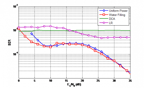
Figure 4 shows the average bitrate per subcarrier for different algorithms including: uniform power allocation with adaptive modulation, Water-filling with adaptive modulation, LR algorithm, and DCA algorithm. Figure 5. shows the average total allocated power per subcarrier, and Figure 6 shows the BER performance for different algorithms.
Figure 4. Average data rate performance for different algorithms
From Figure 4, it can be seen the superiority of the DCA algorithm over all other algorithms. The LF algorithm has a slight lower data rate at medium SNR values. The water-filling power allocation with adaptive modulation gives only a slight improvement for low SNR values in comparison with uniform power allocation.
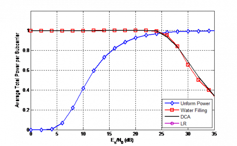
From Figure 5, it can be seen that both DCA and LF algorithm have similar power performance where they use the total available power for SNR below 30dB, then the total power decreases because all active subcarriers are maximally loaded, and the remaining power is insufficient to activate new subcarriers.
Form Figure 6, it can be seen that only the DCA algorithm match exactly the BER threshold, whereas the LF algorithm overestimates the allocated power due the underlying approximations, and the WF algorithm does not optimizes the allocated power discrete bit-load. This results in a lower BER values than the target BER threshold.
Figure 5. Average total power performance for different algorithms
Figure 6. BER performance for different algorithms
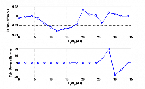
Figure 7 shows the difference in performance between the DCA algorithm and the proposed LC-DCA using the proposed heuristic cost function. It can be seen that the LC-DCA produces a too close solution with very small data rate reduction of 0.04 bits/subcarrier at medium SNR. Sometimes, the difference is positive due to borders effects as it can be seen for SNR=20dB.
Figure 7. Difference of data rate (upper) and average total power (lower) between LC-DCA and DCA
Figure 8. Bit error rate (upper), average allocated bits (middle), average allocated power (lower), for a given non-uniform QoS profile at different SNR values
Finally, Figure 8 shows the ability of the propose algorithm to satisfy different QoS requirements for differen subcarriers. The number of subcarriers is $\mathrm{N}=128$. The BEF threshold is set to $10^{-3}$ for subcarriers $1-64$ with maximun bit-load of 6 bits. For the remaining subcarriers, the BEF threshold is set to and $10^{-4}$ with maximum bit-load of 4 bits Similar results were obtained for a coded system using a rate $1 / 2$ convolutional code.
In this paper, we proposed two different algorithms following two different approaches to solve the optimization problem of data rate maximization in multicarrier system using a discrete modulation set.
• The first algorithm is the LR algorithm which is based on the LR approach. This is a suboptimal algorithm which operates in similar manner as water-filling method with bounded bit-load. It is specific to non-coded systems using a set of M-QAM modulations.
• The second algorithm is the LC-DCA algorithm which is based on discrete linear programming using coordinate ascent framework. This is a suboptimal algorithm which operates in iterative manner. It is a generic algorithm which is suitable for coded as well as non-coded systems with an arbitrary modulation set. This algorithm overcomes the limitation of the HH algorithm with the help of a simple heuristic cost function without scarifying the bitrate performance.
• The performance of the LC-DCA algorithm is better than the performance of the LR algorithm with slightly higher complexity. Future works are directed to extend the obtained results for MIMO system with precoding.
[1] Liu, H., Ma, H., El Zarki, M., Gupta, S. (1997). Error control schemes for networks: An overview. Mobile Networks and Applications, 2: 167-182. https://doi.org/10.1023/A:1013676531988
[2] Hwang, T., Yang, C., Wu, G., Li, S., Ye Li, G. (2009). OFDM and its wireless applications: A survey. IEEE Transactions on Vehicular Technology, 58(4): 1673-1694. https://doi.org/10.1109/TVT.2008.2004555
[3] Fu, I., Chen, Y., Cheng, P., Yuk, Y., Yongho Kim, R., Kwak, J. (2010). Multicarrier technology for 4G WiMax System [WiMAX/LTE Update]. IEEE Communications Magazine, 48(8): 50-58. https://doi.org/10.1109/MCOM.2010.5534587
[4] Liu, K., Tang, B., Liu, Y. (2009). Adaptive power loading based on unequal-BER strategy for OFDM systems. IEEE Communications Letters, 13(7): 474-476. https://doi.org/10.1109/LCOMM.2009.082158
[5] Chow, P.S., Cioffi, J.M., Bingham, J.A.C. (1995). A practical discrete multitone transceiver loading algorithm for data transmission over spectrally shaped channels. IEEE Transactions on Communications, 43(2/3/4): 773-775. https://doi.org/10.1109/26.380108
[6] Mahmood, A., Belfiore, J. (2010). An efficient algorithm for optimal discrete bit-loading in multicarrier systems. IEEE Transactions on Communications, 58(6): 1627-1630. https://doi.org/10.1109/TCOMM.2010.06.0800482
[7] Cioffi, J.M. (1991). A multicarrier primer. Clearfield, USA, Tech. Rep. ANSI Contribution T1E1, 4: 91-157.
[8] Proakis. (2001). Digital Communication Systems, 4th Ed. McGraw Hill.
[9] Wyglinski, A., Labeau, F., Kabal, P. (2005). Bit loading with BER constraint for multicarrier systems. IEEE Transactions on Wireless Communications, 4(4): 1383-1387. https://doi.org/10.1109/TWC.2005.850313
[10] Hughes-Hartogs, D. (1989). Ensemble modem structure for imperfect transmission media. U.S. Patent No. 4679227.
[11] Zhang, H., Fu, J., Song, J. (2010). A Hughes-Hartogs algorithm based bit-loading algorithm for OFDM systems. 2010 IEEE International Conference on Communications, Cape Town, South Africa, pp. 1-5. https://doi.org/10.1109/ICC.2010.5502109
[12] Bedeer, E., Dobre, O.A., Ahmed, M.H., Baddour, K.E. (2012). Optimal bit and power loading for OFDM systems with average BER and total power constraints. IEEE Global Communications Conference (GLOBECOM), Anaheim, CA, pp. 3685-3689. https://doi.org/10.1109/GLOCOM.2012. 6503689
[13] Bedeer, E., Dobre, O.A., Ahmed, M.H., Baddour, K.E. (2015). A systematic approach to jointly optimize rate and power consumption for OFDM systems. IEEE Transactions on Mobile Computing, 15(6): 1305-1317. https://doi.org/10.1109/TMC.2015.2465393
[14] Cormen, T.H., Stein, C., Rivest, R.L., Leiserson, C.E. (2001). Introduction to Algorithms. Higher Education, 2nd edition. McGraw-Hill Inc.
[15] Benson H.P. (1995). Concave Minimization: Theory, Applications and Algorithms. In: Horst R., Pardalos P.M. (eds) Handbook of Global Optimization. Nonconvex Optimization and Its Applications, 2, 43-148. Springer, Boston, MA.
[16] Iraqi, Y., Al-Dweik, A. (2020). Adaptive bit loading with reduced computational time and complexity for multicarrier wireless communications. IEEE Transactions on Aerospace and Electronic Systems, 56(3): 2497-2506. https://doi.org/10.1109/TAES.2019.2946505
[17] De Souza, J.H.I., Abrão, T. (2018). Hybrid Hughes-Hartogs power allocation algorithms for OFDMA systems. IET Signal Processing, 12(9): 1185-1192. https://doi.org/10.1049/iet-spr.2018.5080