Nooh Bany Muhammad | Mubashar Sarfraz | Sajjad A. Ghauri* | Saqib Masood
© 2021 IIETA. This article is published by IIETA and is licensed under the CC BY 4.0 license (http://creativecommons.org/licenses/by/4.0/).
OPEN ACCESS
Automatic modulation classification (AMC) is the emerging research area for military and civil applications. In this paper, M-PSK signals are classified using the optimized polynomial classifier. The distinct features i.e., higher order cumulants (HOC’s) are extracted from the noisy received signal and the dataset is generated with different number of samples, various SNR’s and on several fading channels. The proposed classifier structure classifies the overall modulation classification problem into binary sub-classifications. In each sub-classification, the extracted features are expanded using polynomial expansion into higher dimension space. In higher dimension space numerous non-linearly separable classes becomes linearly separable. The performance of the proposed classifier is evaluated on Rayleigh and Rician fading channels in the presence of additive white gaussian noise (AWGN). The polynomial classifier performance is optimized using one of the famous heuristic computational techniques i.e., Genetic Algorithm (GA). The extensive simulations have been carried with and without optimization, which shows relatively better percentage classification accuracy (PCA) as compared with the state of art existing techniques.
automatic modulation classification, higher order cumulants, polynomial classifier, M-PSK, genetic algorithm
From past few decades, automatic modulation classification (AMC) application in communication systems has been an intriguing area for the researchers. AMC is a process to classify the modulation technique employed in the transmitted signals. AMC is conceded between the detection and demodulation of the received signal [1, 2]. AMC is generally divided into two categories:
The decision-theoretic approach also termed as the likelihood-based approached in which the probability of correct decision is maximize via utilizing prior information. Even though the approach is optimal and high computational complexity. The decision theoretic approach provides optimal solution by calculating the likelihood function of the received signal. After having the likelihood function there are several tests to detect the modulation format such as: average likelihood ratio test (ALRT), generalized likelihood ratio test (GLRT), hybrid likelihood ratio test (HLRT), quasi-likelihood ratio test (Q-ALRT), kullback-leibler divergence test (KLDT) and the detailed explanation of decision theoretic approach can be found in [3-6].
In pattern recognition approach the received signals characteristics are exploited and various parameters are extracted. After extracting the parameters, feature selection is carried out. While comparing to the decision-theoretic approach, feature-based approach is sub-optimal, but with the advantage of reducing computational complexity [7]. The works [8-22] related to feature-based pattern recognition approach have been listed in Table 1. In the literature, authors have been utilized various classifier structures to classify the modulation formats [23, 24]. The classifiers are based on hidden Markov model (HMM), neural network based, support vector machine based, convolutional neural network based, recurrent neural network based, deep neural network based and Gabor filter network [25-28].
In this research, M-PSK signals are considered for classification using polynomial classifier. The polynomial classifier (PC) is optimized using one of the evolutionary computational techniques i.e., Genetic Algorithm. The PC transforms the feature space into higher dimension space (HDS). Various classes in low dimension space are non-linearly separable while in HDS it becomes linearly separable. The performance of PC is evaluated on various channel model and compared with the optimized PC (OPC).
The rest of the paper is organized as follows: In section 2 system model is presented with the extracted features and polynomial classifier structure. Proposed classifier algorithm and the optimization is discussed in Section 3. The detailed simulation is carried out in section 4. In the end, the paper is concluded.
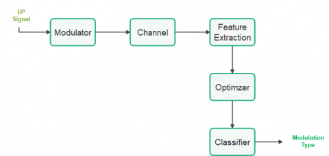
The system model for classification of M-PSK signals is shown in Figure 1. The signals have been considered for classification are PSK-4, PSK-8, PSK-16, PSK-32, and PSK-64. The modulated signal is transmitted over the faded channel (Rayleigh and Rician) with the addition of white gaussian noise. Higher order cumulants (HOCs) are selected as a feature set extracted from the received signal. In the first approach, these features are fed to the polynomial classifier, while in the second approach these features are optimized using Genetic Algorithm and fed to the polynomial classifier structure. The general expression of the received signal can be written as:
$r_{n}=s_{n}+g_{n}$ (1)
where, rn is the received signal, gn is AWGN and sn is the modulated signal.
Figure 1. System model of the proposed algorithm
Table 1. Some existing feature-based techniques
|
Ref. |
Classifier Algorithm |
Modulation Formats |
Channel |
Features |
|
[1] |
Genetic Algorithm |
QAM and PSK |
AWGN |
Spectral |
|
[2] |
Combined GP and KNN |
BPSK, QPSK, QAM16, QAM64 |
AWGN |
Cumulants |
|
[8] |
MAP |
OFDM |
AWGN, Fading |
HOC |
|
[9] |
Pattern |
M-PSK |
Fading |
HOC |
|
[10] |
ML |
BPSK, QPSK, 8PSK, 16QAM |
Rayleigh Fading, AWGN |
High order cyclic cumulants |
|
[11] |
Hierarchical Classifier |
M- ASK, FSK, PSK |
AWGN |
Instantaneous Spectral Feature |
|
[12] |
Linear and non-linear classifier |
BPSK, 4PAM, QPSK, 16QAM, 64QAM |
Multipath flat fading |
HOC |
|
[14] |
Support Vector Machine |
FSK, ASK, PSK |
Fading |
HOC |
|
[15] |
Pattern Recognition |
M-PSK M-QAM |
Flat Fading, |
HOC |
|
[16] |
Artificial Neural Network |
FSK, PSK, PAM, QAM |
Rayleigh Flat Fading and AWGN |
High Order Statistics, Spectral |
|
[17] |
Genetic Programming with KNN |
BPSK, QPSK, 16QAM, 64QAM |
AWGN |
HOC |
|
[18] |
Artificial Neural Network |
PSK, FSK, ASK, AM, FM, DSB |
AWGN |
Statistical, Spectral |
|
[19] |
Pattern Recognition (MLP) |
M-PAM, M-PSK, M-FSK, M-QAM |
AWGN, Rayleigh Flat Fading, |
Cyclo-stationary |
|
[20] |
Pattern Recognition(MPL) |
M-PAM, M-PSK, M-FSK, M-QAM |
AWGN, Rayleigh Flat Fading, Rician Flat Fading |
Spectral |
|
[21] |
Hierarchical Classifier |
M-PSK |
AWGN |
HOC |
2.1 Feature extraction
From the received signal as in Eq. (1), the higher order cumulants are extracted as features set. For this, the pth order moment is defined as: -
$M_{p a}=E\left[r^{p-q}\left(r^{*}\right)^{q}\right]$ (2)
The second order, forth order, sixth order cumulants and 8th order cumulants expressions are expressed as follows [14]:
$\mathrm{C}_{20}=\mathrm{M}_{20}=\mathrm{E}\left[\mathrm{r}^{2}(\mathrm{n})\right]$ (3)
$\mathrm{C}_{21}=\mathrm{M}_{21}=\mathrm{E}\left[|\mathrm{r}(\mathrm{n})|^{2}\right]$ (4)
$\mathrm{C}_{40}=\mathrm{M}_{40}-3 M_{20}^{2}$ (5)
$C_{41}=M_{40}-3 M_{20} M_{21}$ (6)
$C_{42}=M_{42}-\left|M_{20}\right|^{2}-21 M_{21}$ (7)
$\mathrm{C}_{60}=\mathrm{M}_{60}-15 \mathrm{M}_{20} \mathrm{M}_{40}+30 \mathrm{M}_{20}{ }^{3}$ (8)
$C_{61}=M_{61}-15 M_{21} M_{40}-10 M_{20} M_{41}+30 M_{20}^{2} M_{21}$ (9)
$C_{62}=M_{62}-6 M_{20} M_{42}-8 M_{21} M_{41}-M_{22} M_{40}$$+6 M_{20}^{2} M_{22}+24 M_{21}^{2} M_{22}$ (10)
$C_{63}=M_{62}-9 M_{21} M_{42}+12 M_{21}^{3}-3 M_{20} M_{43}$$-3 M_{22} M_{41}+18 M_{20} M_{21} M_{22}$ (11)
$C_{80}=M_{80}-35 M_{40}^{2}-28 M_{60} M_{20}$$+420 M_{40} M_{20}^{2} 630 M_{20}^{4}$ (12)
From the Eqns. (3)-(12), the distinct features are extracted and higher order cumulants have been served as feature set. The features are extracted for different number of samples, different modulation formats, various SNR’s and channel conditions i.e. Rician and Rayleigh.
2.2 Polynomial classifier
The crux of the polynomial classifier is to expand the original features set space into higher dimensional space, where various classes become linearly separable [20]. Generally, there are two stages of PC:
1) Training of PC
2) Testing of PC
2.2.1 Training stage of polynomial classifier
In the training stage, the received signal with known modulation type is used to find the weight vectors. The extracted features are transformed into higher dimensional space using polynomial expansion method to yield more distinct features. This expansion of the features vector allows us the linear separation of the modulation formats. The order of the classifier is same as the dimension of the expanded feature space. Higher order classifiers can be used, but for simplicity and due to ease of implementation generally lower order classifiers have been utilized, however, in this research, the second order polynomial classifier is used. In the second order polynomial classifier, the original extracted features plus the product of these features and squared values of these features have been found. Let Ci is the vector that contains input features which are higher order cumulants [21].
$C_{i}=\left[C_{i, 1}, C_{i, 2}, C_{i, 3}, \ldots C_{i, K}\right]$ (13)
The feature vector Ci is expanded using polynomial expansion and the resulting expanded feature vector Pi is given below:
$P_{i}=\left[C_{i, 1}, C_{i, 2}, C_{i, 3}, \ldots, C_{i, K}, C_{i, 1} \times C_{i, 2}, \ldots, C_{i, 1} \times, C_{i, 2}\right.$$\times C_{i, 3}, \ldots, C_{i, 2} \times C_{i, K}, \ldots, C_{i, K-1}$$\left.\times C_{i, K}, C_{i, 1}^{2}, C_{i, 2}^{2}, \ldots, C_{i, K}^{2}\right]_{1 \times R}$ (14)
The dimension of the expanded feature space is denoted by R, and K represents the total number of the features i.e., HOC. Expansion of features vectors for all N number of classes will result in a matrix G that is produced by concatenating all Pi. For N feature vectors, the expanded feature vectors are $P_{1}, P_{2}, \ldots, P_{N}:$-
$P_{N}=\left[C_{N 1}, C_{N 2}, C_{N 3}, \ldots, C_{N M}\right]$ (15)
$G=\left[P_{1}, P_{2}, \ldots, P_{N}\right]$ (16)
$\mathrm{X}=\mathrm{G}^{\prime} \times \mathrm{G}$ (17)
In the next step, optimized weights are selected to reduce the minimum mean square error as: -
$\mathrm{W}=X^{-1} \times G$ (18)
where, W is the weight vector. The weight is used in the testing stage to recognize the modulation type of the received signal. The block diagram of the training stage of polynomial classifier is shown in Figure 2.
Figure 2. Training stage
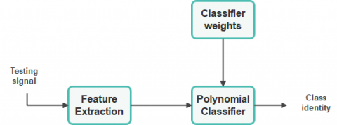
2.2.2 Testing stage of polynomial classifier
In the testing stage, the received signals that have unknown modulation formats are applied to the polynomial classifier to recognize the modulation formats of the received signals. The ith feature vector Ci that contains higher order cumulants is extracted and then ith expanded feature vector Pi is determined using the Eq. (14). The second order polynomial expansion is used, and expanded vector Pi is multiplied with the classifier weights Wi to obtain the scores Si: -
$S_{i}=P_{i} * W_{i}$ (19)
These scores present the new super features for the polynomial classifier and based on these scores, the modulated signal, modulation format is determined. The class identity of vector C is determined by the following rule: -
selected $\left\langle\right.$ class $\left._{i}\right\rangle=\arg \left(\underset{i}{\max }\left\{S_{i}\right\}\right)$ (20)
For example, if there are two modulation types i.e., BPSK and QPSK, then there are two scores S1 and S2. If the score S1 is greater than the S2, then the modulation type is BPSK, otherwise the modulation type is QPSK. The block diagram shown in Figure 3, representing the training stage of polynomial classifier.
Figure 3. Testing stage
|
Algorithm 1: GA based polynomial classifier |
|
Inputs: N → Number of samples M → Modulation order Ub → Upper bound of N Lb → Lower bound of N sn → Modulated signal Cht → Channel type (Rician or Rayleigh) snr → Signal to noise ratio Outputs: return; PCA → Percentage Classification Accuracy Initialization: Initialize; $\forall$ parameters $\forall$ variables |
|
Main:
|
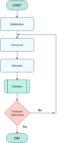
Figure 4. Flow chart of GA
To optimize the classifier performance, the GA is used to optimize the features and to reduce the mean square error by finding the optimized weight vector. The figure of merit of the classification problem is percentage PCA (PCA) which is enhanced by using optimal values of the overexcited parameters. GS is used as global optimization due to their greater efficiency and is stochastic optimization algorithm which adopts the survival of the fittest theory of Darwin. GA is used to take the optimal features and classifier must reject the similar features means redundant features to reduce the computational complexity. The flow chart of the genetic algorithm for classification of modulation formats is shown in Figure 4. The pseudo code of proposed classifier structure is shown.
The performance of polynomial classifier and optimized polynomial classifier have been evaluated for the classification of M-PSK signals. The figure of the merit of the considered problem is percentage classification accuracy (PCA). The simulation parameters are shown in the Table 2. The extensive simulations have been carried out with 512, 1024 and 2048 number of samples and different SNR’s of 0dB, 5dB and 10dB. Two fading channel models have been considered throughout the simulations i.e., Rayleigh and Rician.
Table 2. Simulation parameters
|
Parameters |
Values |
|
Candidate Solutions |
10-50 |
|
Cross-over |
Single Point |
|
Selection |
Roulette Wheel |
|
Mutation |
Adaptive |
|
Classifier |
Polynomial |
|
Iterations |
1000 |
|
SNR in dB |
0-10 |
4.1 Case-1: Classification on Non-Fading Channel Model
The classifier performance is evaluated on non-fading channel i.e., only considered the AWGN. Tables 3-11 shows the PCA for AWGN channel model with different number of samples and SNR’s. From the Tables 3-5, the average PCA for the 512 number of samples is 87.5%, 89.46% and 91.94% at 0, 5 and 10 dB of SNR, respectively.
Table 3. PCA on AWGN Channel at SNR of 0dB, N=512
|
PSK |
4 |
8 |
16 |
32 |
64 |
|
4 |
84.3% |
|
|
|
|
|
8 |
|
92.4% |
|
|
|
|
16 |
|
|
83.8% |
|
|
|
32 |
|
|
|
84.1% |
|
|
64 |
|
|
|
|
93% |
Table 4. PCA on AWGN Channel at SNR of 5dB, N=512
|
PSK |
4 |
8 |
16 |
32 |
64 |
|
4 |
87.3% |
|
|
|
|
|
8 |
|
93.5% |
|
|
|
|
16 |
|
|
86.4% |
|
|
|
32 |
|
|
|
87.1% |
|
|
64 |
|
|
|
|
93% |
Table 5. PCA on AWGN Channel at SNR of 10dB, N=512
|
PSK |
4 |
8 |
16 |
32 |
64 |
|
4 |
88% |
|
|
|
|
|
8 |
|
94.7% |
|
|
|
|
16 |
|
|
88.8% |
|
|
|
32 |
|
|
|
90.2% |
|
|
64 |
|
|
|
|
98% |
Tables 6-8, the PCA improves as number of samples increases from 512 to 1024. The average PCA at 10dB of SNR is 93.9% which is better that 91.94% for 512 number of samples.
Table 6. PCA on AWGN Channel at SNR of 0dB, N=1024
|
PSK |
4 |
8 |
16 |
32 |
64 |
|
4 |
87.3% |
|
|
|
|
|
8 |
|
93.4% |
|
|
|
|
16 |
|
|
90.8% |
|
|
|
32 |
|
|
|
85.1% |
|
|
64 |
|
|
|
|
98.1% |
Table 7. PCA on AWGN Channel at SNR of 5dB, N=1024
|
PSK |
4 |
8 |
16 |
32 |
64 |
|
4 |
88.3% |
|
|
|
|
|
8 |
|
94.4% |
|
|
|
|
16 |
|
|
91.1% |
|
|
|
32 |
|
|
|
89.4% |
|
|
64 |
|
|
|
|
98.5% |
Table 8. PCA on AWGN Channel at SNR of 10dB, N=1024
|
PSK |
4 |
8 |
16 |
32 |
64 |
|
4 |
89.1% |
|
|
|
|
|
8 |
|
95.2% |
|
|
|
|
16 |
|
|
93.8% |
|
|
|
32 |
|
|
|
92.22% |
|
|
64 |
|
|
|
|
99% |
Table 9. PCA on AWGN Channel at SNR of 0dB, N=2048
|
PSK |
4 |
8 |
16 |
32 |
64 |
|
4 |
88.9% |
|
|
|
|
|
8 |
|
95.1% |
|
|
|
|
16 |
|
|
92% |
|
|
|
32 |
|
|
|
89.2% |
|
|
64 |
|
|
|
|
99.45% |
Table 10. PCA on AWGN Channel at SNR of 5dB, N=2048
|
PSK |
4 |
8 |
16 |
32 |
64 |
|
4 |
89% |
|
|
|
|
|
8 |
|
97.2% |
|
|
|
|
16 |
|
|
93.8% |
|
|
|
32 |
|
|
|
92.1% |
|
|
64 |
|
|
|
|
100% |
Table 11. PCA on AWGN Channel at SNR of 10dB, N=2048
|
PSK |
4 |
8 |
16 |
32 |
64 |
|
4 |
92% |
|
|
|
|
|
8 |
|
98.7% |
|
|
|
|
16 |
|
|
94.8% |
|
|
|
32 |
|
|
|
96.2% |
|
|
64 |
|
|
|
|
100% |
Tables 9-11 shows the percent accuracy of classification with 2048 number of samples and average PCA is quite improved as compared with 512 and 1024 number of samples i.e., 96.34%.
4.2 Case-2: Classification on Rician Fading Channel
The classifier performance is evaluated on Rician channel model. Tables 12-20 shows the PCA for Rician channel model with different number of samples and SNR’s. From the Tables 12-14, the average PCA for the 512 number of samples is 86.4%, 88% and 88.26% at 0, 5 and 10 dB of SNR, respectively.
Tables 15-17, the PCA improves as number of samples increases from 512 to 1024. The average PCA at 10dB of SNR is 91.5% which is better that 88.26% for 512 number of samples. Table 18-20 shows the percent accuracy of classification with 2048 number of samples and average PCA is quite improved as compared with 512 and 1024 number of samples i.e., 94.1%.
Table 12. PCA on Rician Channel at SNR of 0dB, N=512
|
PSK |
4 |
8 |
16 |
32 |
64 |
|
4 |
83% |
|
|
|
|
|
8 |
|
91.4% |
|
|
|
|
16 |
|
|
83.7% |
|
|
|
32 |
|
|
|
82.7% |
|
|
64 |
|
|
|
|
91% |
Table 13. PCA on Rician Channel at SNR of 5dB, N=512
|
PSK |
4 |
8 |
16 |
32 |
64 |
|
4 |
85.3% |
|
|
|
|
|
8 |
|
92.66% |
|
|
|
|
16 |
|
|
84.3% |
|
|
|
32 |
|
|
|
86% |
|
|
64 |
|
|
|
|
92% |
Table 14. PCA on Rician Channel at SNR of 10dB, N=512
|
PSK |
4 |
8 |
16 |
32 |
64 |
|
4 |
86.9% |
|
|
|
|
|
8 |
|
93.86% |
|
|
|
|
16 |
|
|
86.34% |
|
|
|
32 |
|
|
|
88.92% |
|
|
64 |
|
|
|
|
95% |
Table 15. PCA on AWGN Channel at SNR of 0dB, N=1024
|
PSK |
4 |
8 |
16 |
32 |
64 |
|
4 |
86.4% |
|
|
|
|
|
8 |
|
92% |
|
|
|
|
16 |
|
|
88.2% |
|
|
|
32 |
|
|
|
84.7% |
|
|
64 |
|
|
|
|
92% |
Table 16. PCA on AWGN Channel at SNR of 5dB, N=1024
|
PSK |
4 |
8 |
16 |
32 |
64 |
|
4 |
87.1% |
|
|
|
|
|
8 |
|
93.4% |
|
|
|
|
16 |
|
|
89.9% |
|
|
|
32 |
|
|
|
87% |
|
|
64 |
|
|
|
|
95.2% |
Table 17. PCA on AWGN Channel at SNR of 10dB, N=1024
|
PSK |
4 |
8 |
16 |
32 |
64 |
|
4 |
88.22% |
|
|
|
|
|
8 |
|
94% |
|
|
|
|
16 |
|
|
90% |
|
|
|
32 |
|
|
|
89.25% |
|
|
64 |
|
|
|
|
96 % |
Table 18. PCA on Rician Channel at SNR of 0dB, N=2048
|
PSK |
4 |
8 |
16 |
32 |
64 |
|
4 |
87% |
|
|
|
|
|
8 |
|
94.5% |
|
|
|
|
16 |
|
|
90.7% |
|
|
|
32 |
|
|
|
88% |
|
|
64 |
|
|
|
|
95% |
Table 19. PCA on Rician Channel at SNR of 5dB, N=2048
|
PSK |
4 |
8 |
16 |
32 |
64 |
|
4 |
88% |
|
|
|
|
|
8 |
|
95% |
|
|
|
|
16 |
|
|
91.1% |
|
|
|
32 |
|
|
|
89% |
|
|
64 |
|
|
|
|
97% |
Table 20. PCA on Rician Channel at SNR of 10dB, N=2048
|
PSK |
4 |
8 |
16 |
32 |
64 |
|
4 |
90% |
|
|
|
|
|
8 |
|
96.9% |
|
|
|
|
16 |
|
|
92.33% |
|
|
|
32 |
|
|
|
92% |
|
|
64 |
|
|
|
|
98.9% |
4.3 Case-3: Classification on Rayleigh Fading Channel
The classifier performance is evaluated on Rayleigh channel model. Tables 21-29 shows the PCA for Rayleigh channel model with different number of samples and SNR’s. The average PCA for 512, 1024 and 2048 number of samples at 10dB of SNR is 88.5%, 90.1% and 92.14%. The average PCA is slightly less at 5 dB and 0dB of SNR and can be seen from the tables 21-23, 24-26, 27-29.
Table 21. PCA on Rayleigh Channel at SNR of 0dB, N=512
|
PSK |
4 |
8 |
16 |
32 |
64 |
|
4 |
81.98% |
|
|
|
|
|
8 |
|
90% |
|
|
|
|
16 |
|
|
81.7% |
|
|
|
32 |
|
|
|
82% |
|
|
64 |
|
|
|
|
90% |
Table 22. PCA on Rayleigh Channel at SNR of 5dB, N=512
|
PSK |
4 |
8 |
16 |
32 |
64 |
|
4 |
83.7% |
|
|
|
|
|
8 |
|
91.5% |
|
|
|
|
16 |
|
|
82.8% |
|
|
|
32 |
|
|
|
85.7% |
|
|
64 |
|
|
|
|
91.3% |
Table 23. PCA on Rayleigh Channel at SNR of 10dB, N=512
|
PSK |
4 |
8 |
16 |
32 |
64 |
|
4 |
84.8% |
|
|
|
|
|
8 |
|
92% |
|
|
|
|
16 |
|
|
84.3% |
|
|
|
32 |
|
|
|
87% |
|
|
64 |
|
|
|
|
94.5% |
Table 24. PCA on Rayleigh Channel at SNR of 0dB, N=1024
|
PSK |
4 |
8 |
16 |
32 |
64 |
|
4 |
85% |
|
|
|
|
|
8 |
|
91% |
|
|
|
|
16 |
|
|
86.9% |
|
|
|
32 |
|
|
|
83% |
|
|
64 |
|
|
|
|
91% |
Table 25. PCA on Rayleigh Channel at SNR of 5dB, N=1024
|
PSK |
4 |
8 |
16 |
32 |
64 |
|
4 |
85.56% |
|
|
|
|
|
8 |
|
92% |
|
|
|
|
16 |
|
|
87% |
|
|
|
32 |
|
|
|
85.6% |
|
|
64 |
|
|
|
|
93% |
Table 26. PCA on Rayleigh Channel at SNR of 10dB, N=1024
|
PSK |
4 |
8 |
16 |
32 |
64 |
|
4 |
86% |
|
|
|
|
|
8 |
|
93.6% |
|
|
|
|
16 |
|
|
88.96% |
|
|
|
32 |
|
|
|
87% |
|
|
64 |
|
|
|
|
95.1% |
Table 27. PCA on Rayleigh Channel at SNR of 0dB, N=2048
|
PSK |
4 |
8 |
16 |
32 |
64 |
|
4 |
85.5% |
|
|
|
|
|
8 |
|
93% |
|
|
|
|
16 |
|
|
88.9% |
|
|
|
32 |
|
|
|
85% |
|
|
64 |
|
|
|
|
91.8% |
Table 28. PCA on Rayleigh Channel at SNR of 5dB, N=2048
|
PSK |
4 |
8 |
16 |
32 |
64 |
|
4 |
86% |
|
|
|
|
|
8 |
|
94% |
|
|
|
|
16 |
|
|
90.6% |
|
|
|
32 |
|
|
|
87% |
|
|
64 |
|
|
|
|
95% |
Table 29. PCA on Rayleigh Channel at SNR of 10dB, N=2048
|
PSK |
4 |
8 |
16 |
32 |
64 |
|
4 |
88% |
|
|
|
|
|
8 |
|
95% |
|
|
|
|
16 |
|
|
91% |
|
|
|
32 |
|
|
|
90% |
|
|
64 |
|
|
|
|
96.7% |
4.4 Case-4: Classification Performance Comparison
Table 30 shows the comparison of PCA of polynomial classifier and optimized polynomial classifier at 0dB of SNR. From the table, it is evident that after optimization, there is a significant improvement in PCA as compared without optimization. The PCA is 98% of OPC while 92.8% of PC for AWGN channel model at 2048 number of samples.
Table 30. PCA after Optimization Comparison at SNR of 0dB
|
|
Samples |
SNR in dB |
||
|
0 |
5 |
10 |
||
|
AWGN |
512 |
89.3% |
91% |
92.5% |
|
1024 |
93.6% |
96% |
97% |
|
|
2048 |
98% |
99.1% |
99.8% |
|
|
Rician |
512 |
88.8% |
90.1% |
91.9% |
|
1024 |
92% |
93.5% |
94.9% |
|
|
2048 |
95% |
96.7% |
98.9% |
|
|
Rayleigh |
512 |
87% |
88.6% |
91% |
|
1024 |
91.5% |
95% |
97.1% |
|
|
2048 |
93% |
95% |
97% |
|
Table 31. Comparison of proposed algorithm with the existing techniques
|
Samples |
SNR (dB) |
Native |
SVM |
GP-KNN |
Without optimization |
With optimization |
|
512 |
0 |
63% |
64% |
65% |
87% |
89% |
|
10 |
90% |
91% |
94% |
91.9% |
92.5% |
|
|
1024 |
0 |
69% |
70% |
70% |
90% |
93.6% |
|
10 |
94% |
94% |
97% |
93% |
97% |
|
|
2048 |
0 |
76% |
75% |
95% |
92% |
98% |
|
10 |
97% |
97% |
98% |
96% |
99.9% |
In Table 31, the performance of proposed optimized polynomial classifier is compared with the well-known existing techniques and from the table, proposed OPC performs better in terms of percentage classification accuracy. The PCA is evaluated for different number of samples as well as different SNR’s. The PCA is around 98% even at lower SNR’s.
In this paper, an optimized polynomial classifier is employed to classify M-PSK signals. From the noisy received signal, HOCs are extracted and these feature vectors are fed into the polynomial classifier. The polynomial classifier expands the feature vector into a higher dimensional space in which various classes becomes linearly separable. The performance of the classifier is analyzed on Rician and Rayleigh fading channels in addition to white gaussian noise. The performance of classifier is also optimized using a Genetic Algorithm in conjunction with a polynomial classifier. From the extensive simulations, it is shown the supremacy of the proposed classifier as compared with the state of art existing techniques.
[1] Dutta, T., Satija, U., Ramkumar, B., Manikandan, M.S. (2016). A novel method for automatic modulation classification under non-Gaussian noise based on variational mode decomposition. 2016 Twenty Second National Conference on Communication (NCC), pp. 1-6. https://doi.org/10.1109/ncc.2016.7561103.
[2] Aslam, M.W., Zhu, Z., Nandi, A.K. (2012). Automatic modulation classification using combination of genetic programming and KNN. IEEE Transactions on Wireless Communications, 11(8): 2742-2750. https://doi.org/10.1109/twc.2012.060412.110460
[3] Wang, F., Wang, X. (2010). Fast and robust modulation classification via Kolmogorov-Smirnov test. IEEE Transactions on Communications, 58(8): 2324-2332. https://doi.org/10.1109/tcomm.2010.08.090481
[4] Ramezani-Kebrya, A., Kim, I.M., Kim, D.I., Chan, F., Inkol, R. (2013). Likelihood-based modulation classification for multiple-antenna receiver. IEEE Transactions on Communications, 61(9): 3816-3829. https://doi.org/10.1109/tcomm.2013.073113.121001
[5] Headley, W.C., Chavali, V.G., da Silva, C.R.C.M. (2013). Maximum-likelihood modulation classification with incomplete channel information. 2013 Information Theory and Applications Workshop (ITA), pp. 1-4. https://doi.org/10.1109/ita.2013.6503000
[6] Dobre, O.A., Abdi, A., Bar-Ness, Y., Su, W. (2007). Survey of automatic modulation classification techniques: Classical approaches and new trends. IET Communications, 1(2): 137-156. https://doi.org/10.1049/iet-com:20050176
[7] Satija, U., Mohanty, M., Ramkumar, B. (2015). Automatic modulation classification using S-transform based features. 2015 2nd International Conference on Signal Processing and Integrated Networks (SPIN), pp. 708-712. https://doi.org/10.1109/SPIN.2015.7095322
[8] Hazza, A., Shoaib, M., Alshebeili, S.A., Fahad, A. (2013). An overview of feature-based methods for digital modulation classification. In 2013 1st International Conference on Communications, Signal Processing, and Their Applications (ICCSPA), pp. 1-6. https://doi.org/10.1109/iccspa.2013.6487244
[9] Han, Y., Wei, G., Song, C., Lai, L. (2012). Hierarchical digital modulation recognition based on higher-order cumulants. 2012 Second International Conference on Instrumentation, Measurement, Computer, Communication and Control, pp. 1645-1648. https://doi.org/10.1109/imccc.2012.398
[10] Dobre, O.A., Bar-Ness, Y., Su, W. (2003). Higher-order cyclic cumulants for high order modulation classification. IEEE Military Communications Conference (MILCOM), 1: 112-117. https://doi.org/10.1109/milcom.2003.1290087
[11] Chou, Z.D., Jiang, W.N., Xiang, C.B., Li, M. (2013). Modulation recognition based on constellation diagram for M-QAM signals. 11th IEEE International Conference on Electronic Measurement & Instruments, 1(1): 70-74. https://doi.org/10.1109/ICEMI.2013.6743041
[12] Shah, S.I.H., Alam, S., Ghauri, S.A., Hussain, A., Ansari, F.A. (2019). A novel hybrid Cuckoo search-extreme learning machine approach for modulation classification. IEEE Access, 7: 90525-90537. https://doi.org/10.1109/access.2019.2926615
[13] Ghauri, S.A., Qureshi, I.M., Malik, A.N. Cheema, T.A. (2013). Higher order cummulants based digital modulation recognition scheme. Research Journal of Applied Sciences Engineering & Technology (RJASET), 6(20): 3910-3915. https://doi.org/10.19026/rjaset.6.3609
[14] Ghauri, S.A., Qureshi, I.M., Malik, A.N., Cheema, T.A. (2014). Automatic digital modulation recognition technique using higher order cummulants on faded channels. Journal of Basic and Applied Scientific Research, 4(3): 1-12.
[15] Ghauri, S.A., Qureshi, I.M., Adnan, A., Cheema, T.A. (2014). Classification of digital modulated signals using linear discriminant analysis on faded channel. World Applied Sciences Journal, 29(10):1220-1227. https://doi.org/10.5829/idosi.wasj.2014.29.10.1540
[16] Aslam, M.W., Zhu, Z., Nandi, A.K. (2011). Robust QAM classification using Genetic programming and fisher criterion. 19th European Signal Processing Conference, pp. 995-999.
[17] Liu, A., Zhu, Q. (2011). Automatic modulation classification based on the combination of clustering and neural network. The Journal of China Universities of Posts and Telecommunications, 18(4): 13-38. https://doi.org/10.1016/S1005-8885(10)60077-5
[18] Satija, U., Manikandan, M.S., Ramkumar, B. (2014). Performance study of cyclostationary based digital modulation classification schemes. 9th International Conference on Industrial and Information Systems (ICIIS). pp. 1-5. https://doi.org/10.1109/ICIINFS.2014.7036609
[19] Chen, J., Wang, Y., Wang, D. (2014). A feature study for classification-based speech separation at low signal-to-noise ratios. IEEE/ACM Transactions on Audio, Speech, and Language Processing, 22(12): 1993-2002. https://doi.org/10.1109/TASLP.2014.2359159
[20] Abdelmutalab, A., Assaleh, K., El-Tarhuni, M. (2016). Automatic modulation classification based on high order cumulants and hierarchical polynomial classifiers. Physical Communication, 21: 10-18. https://doi.org/10.1016/j.phycom.2016.08.001
[21] Abdelmutalab, A.E. (2015). Learning-based automatic modulation classification. Ph.D. dissertation.
[22] Abdelmutalab, A., Assaleh, K., El-Tarhuni, M. (2014). Automatic modulation classification using polynomial classifiers. 25th Annual International Symposium on Personal, Indoor, and Mobile Radio Communication (PIMRC), pp. 806-810. https://doi.org/10.1109/PIMRC.2014.7136275
[23] Shah, M.H., Dang, X. (2019). An effective approach for low-complexity maximum likelihood based automatic modulation classification of STBC-MIMO systems. Frontiers of Information Technology & Electronic Engineering, 21: 465-475. https://doi.org/10.1631/fitee.1800306
[24] Im, C., Ahn, S., Yoon, D. (2020). Modulation classification based on Kullback-Leibler divergence. 2020 IEEE 15th International Conference on Advanced Trends in Radioelectronics, Telecommunications and Computer Engineering (TCSET), pp. 373-376. https://doi.org/10.1109/tcset49122.2020.235457
[25] Ghauri, S.A., Qureshi, I.M., Malik, A.N. (2017). A Novel Approach for automatic modulation classification via hidden Markov models and Gabor features. Wireless Personal Communications, 96(3): 4199–4216. https://doi.org/10.1007/s11277-017-4378-x
[26] Meng, F., Chen, P., Wu, L., Wang, X. (2018). Automatic modulation classification: A deep learning enabled approach. IEEE Transactions on Vehicular Technology, 67(11): 10760-10772. https://doi.org/10.1109/tvt.2018.2868698
[27] Ghauri, S.A., Qureshi, I.M., Cheema, T.A., & Malik, A.N. (2014). A novel modulation classification approach using Gabor filter network. The Scientific World Journal, 2014: 643671. https://doi.org/10.1155/2014/643671
[28] Ghauri, S.A. Sarfraz M. Muhammad N.B. Munir, S. (2020). Genetic algorithm assisted support vector machine for M-QAM classification. Mathematical Modelling of Engineering Problems, 7(3): 441-449. https://doi.org/10.18280/mmep.070315