Amirouche Elyazid* | Iffouzar Koussaila | Aouzellag Djamal | Ghedamsi Kaci
© 2021 IIETA. This article is published by IIETA and is licensed under the CC BY 4.0 license (http://creativecommons.org/licenses/by/4.0/).
OPEN ACCESS
This paper presents a standalone tidal stream system with a focus on the reduction of the number of sensors needed by the control scheme. The electromechanical converter is a dual star permanent magnet synchronous generator (DS-PMSG) driven by a horizontal axis marine current turbine (MCT). The generator is controlled via a field oriented control (FOC) strategy and feeds a two three phase two level SVPWM converters, the speed and the position of the shaft are estimated using an extended Kalman filter (EKF), and the speed is regulated using a fuzzy logic controller. The system is simulated using Matlab/Simulink environment, the simulation results show the efficacy of the proposed control scheme, fuzzy speed regulator and the EKF estimator, however, the high number of pole pairs of the generator amplifies the position estimation error even if it was negligible, causing tracking errors of the electromagnetic torque and undesirable high d axis current, but the stability of the system is not affected.
dual star permanent magnet synchronous generator, extended Kalman filter, field oriented control, fuzzy logic controller, marine current turbine
Extracting energy from the flowing sea water is a new form of renewable energy which seems to be promising, essentially due to the high predictability of the tidal current velocities and the high density of the sea water [1, 2], also, the exploitable global tidal energy potential has been estimated to be larger than 100 GW [3].
However, the harsh characteristics of underwater world slow down the developments in this field, so low maintenance high reliability systems are highly recommended to help the development in this area. One of the strategies used for this purpose is the use of multiphase machines made possible thanks to the development of power electronics. They possess several advantages over their three phase counterparts, such as lower torque repulsion, fault tolerance and power segmentation [4, 5]. Another strategy is the exploitation of permanent magnet synchronous generators (PMSG) since they offer higher volumetric torque, lower maintenance need and better efficiency [5]. One of the widely used PMSG multiphase topology is the dual star structure, where the phases are divided into multiple three phase sets, shifted by thirty electrical degrees with isolated neutral points.
The field oriented control (FOC) is often used in many works to successfully control a dual star machine such as in ref. [6, 7], it aims to impose the direction of the fluxes inside an electric machine to get a decoupled control of the flux and torque as in DC machines by using an appropriate transformed model of the controlled device [6]. In Ref. [7, 8] authors used a machine model known as double d-q winding, where each star is replaced by an equivalent d-q winding with a complex mutual coupling between the two pairs, which complicates the machine equations and decreases the dynamic performance of the system. By applying a second consecutive transformation to the aforementioned model, the mutual coupling between the two d-q winding pairs can be eliminated, the obtained model is known as decoupled d-q model [9]. The authors in paper [10] exploited the latter to resolve most problems encountered with the previously mentioned works. Another decoupled model can be found in the literature named extended d-q model [11], which needs only one transformation to successfully decouple the machine equations, which is used in the elaboration of the present paper.
The FOC requires by nature the use of a position encoder mounted on the machine’s shaft to perform the coordinate transformation, which represents the major drawback of this strategy. Using more sensors in the control scheme increases the financial cost and reduces the system’s robustness and reliability, as they are often subject to faults and inaccuracies, especially those mounted in moving parts like speed sensors [12]. To limit these issues, many works focused on technics to reduce sensors number used in the system, such as [13-15]. In this scope of sensorless control strategy, the rotor speed and position are estimated using an EKF, this estimator is widely used in DTC control schemes [16], FOC for three phase synchronous machines [17], and dual star induction motors [18]. In this paper, the EKF is employed to estimate the speed and position of a DS-PMSG allowing to overcome the FOC major drawback.
In this scope, this paper presents a standalone tidal stream system feeding a DC resistive load, with a focus on low maintenance high efficiency devices and control strategies, thus, sensorless strategy is adopted which permits the use of as low number of sensors as possible in order to get a more reliable system, the mathematical modeling of each system part is presented, and advanced control strategies are employed. It is organized into six sections: in the second section a general system description is presented. The third section consists of the mathematical models of the system parts, such as the resource, the turbine and the generator. In the fourth section the control strategy of the machine side converter (MSC) is presented. The simulation results, analysis and discussions are reported in the fifth section. Finally, conclusions about the work are provided in the sixth section.
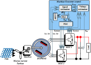
The Figure 1 shows a general scheme of the studied system.
Figure 1. General scheme of the studied system
The generator is driven by a horizontal axis marine current turbine through a gearbox. The use of a gearbox is inevitable in this work because the available machine has only eleven pairs of poles, consequently, an ideal gearbox is integrated in the control scheme. Two three phase two level PWM rectifiers are connected to the machine’s terminals where the outputs are connected in parallel to create a single DC bus feeding a standalone DC resistive load, the two rectifiers are controlled using a sensorless space vector modulated FOC. The speed reference is generated from MPPT, and a new developed fuzzy controller is used to adjust the speed of the turbine.
3.1 Resource modeling
Tidal energy is mainly induced by gravitational interactions between the sun, the earth and the moon. Since the comportment of the sun and the moon is periodic and can be forecasted for decades, the tidal currents are also periodic and highly predictable with an accuracy up to 98% [1]. Some weather conditions can influence tidal currents, such as wind and swell.
A first order model of the tidal current velocity can be derived if the tides coefficient, neap tide and spring tide velocities are known [19].
$v_{t}=V_{n t}+\frac{(C-45)\left(V_{s t}-V_{n t}\right)}{95-45}$ (1)
where, $V_{n t}$ and $V_{s t}$ are the neap tide and spring tide velocities respectively, C is the tides coefficient, 95 and 45 are respectively the spring and neap tides medium coefficients. Using Eq. (1), the tide velocity can be calculated each hour.
3.2 Turbine modeling
Same as for wind energy systems [20], a turbine is used to harness the kinetic power of tidal currents. The horizontal axis turbine is the most used turbine concept in marine energy and wind energy conversion systems. Since it uses the aerodynamic lift effect to operate, this device permits a higher efficiency than devices using aerodynamic drag effect like the vertical axis turbine [21].
The power extracted by a horizontal axis turbine is given as follow:
$P_{t}=\frac{\pi}{2} \rho C_{p} R^{2} v_{t}^{3}$ (2)
where, $R$ is the turbine radius, $\rho$ the sea water density, $v_{t}$ the tide velocity, and $C_{p}$ the power coefficient of the turbine.
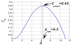
The coefficient $C_{p}$ translates the aerodynamic characteristics of the turbine, it's expressed by the mean of the tip speed ratio (TSR) $\lambda$ and the pitch angle $\beta .$ Its can be defined as a function or a look-up table, the second approach is presented here for a fixed pitch turbine, hence, $C_{p}$ depends only on $\lambda$. The Figure 2 below shows the power coefficient as a function of the TSR of a horizontal axis MCT used in Ref. [22], note that the maximum value of the power coefficient is $0.45$, and the optimal value of the $\mathrm{TSR}$ is $\lambda_{o p t}=6.3$. The other parameters of the turbine are presented in the appendix.
Figure 2. Cp characteristic of a horizontal axis MCT
The TSR is given as:
$\lambda=\frac{\Omega_{t} R}{v_{t}}$ (3)
where, $\Omega_{t}$ is the mechanical angular speed of the turbine.
3.3 Generator modeling
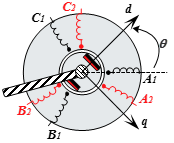
To convert the mechanical power harnessed by the turbine into electricity, a Dual Star PMSG (DSPMSG) is employed. Figure 3 shows the coils configuration of the generator.
Figure 3. Dual star permanent magnet synchronous machine
The stator is composed of two wye-connected stars with isolated neutral points, the two stars are shifted by 30 electrical degrees in respect to each other. To simplify the modeling of this machine, several assumptions are made: all the sets are identical, and the windings are sinusoidally distributed around the air gap, mutual leakage inductances, saturation and eddy currents are not considered.
Many modeling technics are proposed in the literature, in this paper, the extended d-q model is exploited. This model describes the machine by the mean of two decoupled sub-machines, the first, is responsible for the torque and flux generation, the fundamental components and the harmonics of order 12k±1 (k = 1, 2, 3, ...) are mapped into this sub-machine. The second describes the losses, the harmonics of order 6(2k+1)±1 (k = 0, 1, 2, ...) are mapped into this sub-machine [11].
The unbalanced power sharing between the stars caused by the non-idealities and asymmetries in the machine is a well known topic in the literature [7, 11, 23], this unbalance causes non-zero currents to appear in the second sub-machine, to force a balanced power sharing, PI regulators must be used to maintain the currents of this sub-machine equal to zero.
As reported previously in paper [24], using the transformation matrix (4), the simplified mathematical model of a non salient machine can be written as (5):
$T_{p}(\theta)=\frac{1}{\sqrt{2}}\left[\begin{array}{lc}T(\theta) & T\left(\theta-\frac{\pi}{6}\right) \\ T(\theta) & -T\left(\theta-\frac{\pi}{6}\right)\end{array}\right]$ (4)
where
$T(\theta)$$=\sqrt{\frac{2}{3}}\left[\begin{array}{ccc}\cos (\theta) & \cos \left(\theta-\frac{2 \pi}{3}\right) & \cos \left(\theta+\frac{2 \pi}{3}\right) \\ -\sin (\theta) & -\sin \left(\theta-\frac{2 \pi}{3}\right) & -\sin \left(\theta+\frac{2 \pi}{3}\right)\end{array}\right]$$\left\{\begin{array}{c}\frac{d i_{n d}}{d t}=\frac{1}{L_{n d}}\left(v_{n d}-r_{s} i_{n d}+\omega_{e} L_{n q} i_{n q}\right) \\ \frac{d i_{n q}}{d t}=\frac{1}{L_{n q}}\left(v_{n q}-r_{s} i_{n q}-\omega_{e} L_{n d} i_{n d}-\omega_{e} \sqrt{3} \Psi_{P M}\right) \\ \frac{d i_{a d}}{d t}=\frac{1}{L_{a d}}\left(v_{a d}-r_{s} i_{a d}+\omega_{e} L_{a q} i_{a q}\right) \\ \frac{d i_{a q}}{d t}=\frac{1}{L_{a q}}\left(v_{a q}-r_{s} i_{a q}-\omega_{e} L_{a d} i_{a d}\right)\end{array}\right.$ (5)
In this equation set, the terms $L_{x}(x=n d, n q, a d$ or $a q)$ are the cyclic inductances of the machine given in Eq. (6), $\Psi_{P M}$ is the magnitude of the permanent magnet flux, $r_{s}$ the resistance of each stator coil, and $\omega_{e}$ is the electric frequency of the currents in $\mathrm{rad} / \mathrm{s}$.
$\left\{\begin{array}{c}L_{a d}=L_{a q}=L_{s 0}-m \\ L_{n d}=L_{n q}=L_{s 0}+2 m\end{array}\right.$ (6)
$L_{s 0}$ is a constant average value and $m$ the stator magnetizing inductance.
The mechanical behaviour of the machine is described by (7)
$J \frac{d \Omega}{d t}=T_{m}-T_{e m}-f \Omega$ (7)
where, $\omega_{e}=P \Omega$ the electrical frequency, $J$ the total inertia of the system, $\Omega$ the mechanical angular speed of the machine, $T_{m}$ the mechanical torque applied by the turbine on the machine shaft, and $T_{e m}$ the electromagnetic torque developed by the machine given as:
$T_{e m}=P\left(\varphi_{n d} i_{n q}-\varphi_{n q} i_{n d}+\varphi_{a d} i_{a q}-\varphi_{a q} i_{a d}\right)$ (8)
This equation can be simplified leading to:
$T_{e m}=\sqrt{3} P \Psi_{P M} i_{n q}$ (9)
4.1 Field oriented control
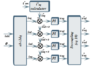
In the Eq. (9), one can see that the current responsible for the torque production is only $i_{n q}$, thus, to get a maximum torque in a non salient machine, this current component must be maximized. The component $i_{n d}$, responsible for the flux production, have to be fixed to zero to assure a good power transmission with minimum losses and to void the magnetic circuit saturation in normal operating conditions. The Figure 4 shows a general scheme of the FOC strategy.
Figure 4. Control scheme of the FOC strategy
In this control scheme, the measured currents of the machine are transformed to the synchronous rotating reference frame using transformation matrix (4), then, using four PI controllers, these currents are regulated to match their reference values. To guarantee a balanced power sharing between the stars and to reduce the current harmonics, the currents references of the second sub-machine $\left(i_{a d}^{*}, i_{a q}^{*}\right)$ are fixed to zero, the current $i_{n d}^{*}$ responsible for flux production is also fixed to zero.
The torque reference is generated by a fuzzy logic speed controller, then the current reference $i_{n q}^{*}$ is calculated using Eq. (9).
The outputs of the PI regulators are the voltage references in the synchronous rotating reference frame. As can be seen in equation set (5), a coupling is present between the d and q components of each sub-machine, eliminating this effect will result in an improved PI controllers’ performance, to perform this decoupling, the terms responsible for the coupling effect are eliminated from the Eq. (5) by adding the decoupling terms (10) to the output of each PI regulator.
$\left\{\begin{array}{c}v_{n d}^{\prime}=\omega_{e} L_{n q} i_{n q} \\ v_{n q}^{\prime}=-\omega_{e} L_{n d} i_{n d}-\omega_{e} \sqrt{3} \Psi_{P M} \\ v_{a d}^{\prime}=\omega_{e} L_{a q} i_{a q} \\ v_{a q}^{\prime}=-\omega_{e} L_{a d} i_{a d}\end{array}\right.$ (10)
The voltage references are used as input to the PWM space vector modulator to generate the control signals for each rectifier.
Instead of measuring the terminal voltage, it is estimated based on the switching states and the DC link voltage using the following equations with $i=1,2$:
$\left[\begin{array}{c}v_{a i} \\ v_{b i} \\ v_{c i}\end{array}\right]=\frac{V_{d c}}{3}\left[\begin{array}{ccc}2 & -1 & -1 \\ -1 & 2 & -1 \\ -1 & -1 & 2\end{array}\right]\left[\begin{array}{c}S_{a i} \\ S_{b i} \\ S_{c i}\end{array}\right]$ (11)
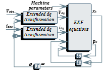
4.2 Extended Kalman filter
The Kalman filter is an optimal estimation algorithm adapted for linear systems, it’s widely used to estimate a system state that cannot be directly measured based on measurable states and the discrete time model of the considered system. For non linear systems, the EKF is employed.
A general equation for a discrete time nonlinear system is given as:
$\left\{\begin{array}{c}x_{k}=f\left(x_{k-1}, u_{k}\right)+w_{k} \\ y_{k}=g\left(x_{k}\right)+v_{k}\end{array}\right.$ (12)
where, $w_{k}$ and $v_{k}$ assumed to be zero mean Gaussian distributions describe the uncertainties and noise related to the system and the measurement respectively. The covariance matrices related to these distributions are denoted $Q$ and $R$ respectively. Note that the system state or the measurement or both can be nonlinear.
In a nonlinear system, contrary to a linear one, the distributions $w_{k}$ and $v_{k}$ can not conserve there Gaussian property after applying the nonlinear function, thus, the Kalman filter can not converge. To conserve the Gaussian properties of these distributions, the EKF linearizes the nonlinear function near the currently state estimation, the linearization is done locally at every time step. The Jacobian matrix is used to linearize the system, it can either be calculated online (numerically) or offline (analytically), the latter is preferred when it’s possible since it improves the computational cost.
The DSPMSM equations calculated earlier in section 3.3 can be rewritten as in Eq. (13):
$\frac{d[x]}{d t}=\left[\begin{array}{ccccc}-\frac{r_{s}}{L_{n d}} & \omega_{e} \frac{L_{n q}}{L_{n d}} & 0 & 0 & 0 \\ -\omega_{e} \frac{L_{n d}}{L_{n q}} & -\frac{r_{s}}{L_{n q}} & 0 & 0 & -\sqrt{3} \frac{\Psi_{P M}}{L_{n q}} \\ 0 & 0 & -\frac{r_{s}}{L_{a d}} & \omega_{e} \frac{L_{a q}}{L_{a d}} & 0 \\ 0 & 0 & -\omega_{e} \frac{L_{a d}}{L_{a q}} & -\frac{r_{s}}{L_{a q}} & 0 \\ 0 & -\frac{\sqrt{3} P^{2}}{J} \Psi_{P M} & 0 & 0 & -\frac{f}{J}\end{array}\right]$$[x]+\left[\begin{array}{cccc}\frac{1}{L_{n d}} & 0 & 0 & 0 \\ 0 & \frac{1}{L_{n q}} & 0 & 0 \\ 0 & 0 & \frac{1}{L_{a d}} & 0 \\ 0 & 0 & 0 & \frac{1}{L_{a q}} \\ 0 & 0 & 0 & 0\end{array}\right][u]$(13)
with, $[x]=\left[\begin{array}{lllll}i_{n d} & i_{n q} & i_{a d} & i_{a q} & \omega_{e}\end{array}\right]^{t}$, and $[u]=\left[\begin{array}{llll}v_{n d} & v_{n q} & v_{a d} & v_{a q}\end{array}\right]^{t}$.
In this equation, the turbine torque $T_{m}$ characterizes an external perturbation, and has not been considered, because the last line of the system will be reduced to zero using a simplification assumption in what follows.
Using the Euler discretization, the system above can be rewritten in discrete time, leading to the following form:
$\left\{\begin{array}{c}x_{k+1}=x_{k}+T_{s} f\left(x_{k}, u_{k}\right) \\ y_{k}=C_{k} u_{k}\end{array}\right.$ (14)
In our case, the system measurement is linear, with
$C_{k}=\left[\begin{array}{lllll}1 & 0 & 0 & 0 & 0 \\ 0 & 1 & 0 & 0 & 0 \\ 0 & 0 & 1 & 0 & 0 \\ 0 & 0 & 0 & 1 & 0\end{array}\right]$
In order to improve the computational cost of the system, the Jacobian is calculated analytically. The system (14) can be expressed by the mean of the Jacobian like shown in Eq. (15). As the discrete sample interval is much smaller compared to the mechanical dynamic of the machine, the model can be simplified by assuming an infinite inertia, hence, the last line of the matrix $A_{k}$ can be reduced to zero.
$x_{k+1}=A_{k} x_{k}+B_{k} u_{k}$ (15)
where,
$A_{k}=I+T_{s}$$\left[\begin{array}{ccccc}-\frac{r_{s}}{L_{n d}} & \omega_{e} \frac{L_{n q}}{L_{n d}} & 0 & 0 & i_{n q} \frac{L_{n q}}{L_{n d}} \\ -\omega_{e} \frac{L_{n d}}{L_{n q}} & -\frac{r_{s}}{L_{n q}} & 0 & 0 & -\left(\begin{array}{c}i_{n d} \frac{L_{n d}}{L_{n q}} \\ +\frac{\sqrt{3} \Psi_{P M}}{L_{n q}}\end{array}\right) \\ 0 & 0 & -\frac{r_{s}}{L_{a d}} & \omega_{e} \frac{L_{a q}}{L_{a d}} & i_{a q} \frac{L_{a q}}{L_{a d}} \\ 0 & 0 & -\omega_{e} \frac{L_{a d}}{L_{a q}} & -\frac{r_{s}}{L_{a q}} & -i_{a d} \frac{L_{a d}}{L_{a q}} \\ 0 & 0 & 0 & 0 & 0\end{array}\right]$
$B_{k}=T_{s}\left[\begin{array}{ccccc}\frac{1}{L_{n d}} & 0 & 0 & 0 & 0 \\ 0 & \frac{1}{L_{n q}} & 0 & 0 & 0 \\ 0 & 0 & \frac{1}{L_{a d}} & 0 & 0 \\ 0 & 0 & 0 & \frac{1}{L_{a q}} & 0 \\ 0 & 0 & 0 & 0 & 0\end{array}\right]$
The Kalman filter operates in two steps, in the first step, called prediction step, a priori state estimation is calculated using the Eq. (16) based on the discrete time model of the system, where the symbol $\hat{x}$ denotes the estimated state, the indices $k-1$ and $k$ denotes the previous and actual step respectively, then, the estimation covariance matrix $\widehat{p_{k}}$ of the estimated state is calculated using Eq. (17).
$\widehat{x_{k}}=A_{k-1} x_{k-1}+B_{k} u_{k}$ (16)
$\widehat{p_{k}}=A_{k-1} \widehat{p_{k-1}} A_{k-1}^{T}+Q$ (17)
In the second step, called measurement update step, the algorithm calculates the Kalman gain $p_{k}$ (Eq. (18)), and uses it to update the predicted state using feedback from the output of the real system as demonstrated by Eq. (19).
After that, the actual state covariance matrix $K_{k}$ is calculated using Eq. (20).
$K_{k}=\frac{\widehat{p_{k}} C_{k}^{T}}{C_{k} \widehat{p_{k}} C_{k}^{T}+R}$ (18)
$x_{k}=\widehat{x_{k}}+K_{k}\left(y_{k}-C_{k} \widehat{x_{k}}\right)$ (19)
$p_{k}=\left(I-K_{k} C_{k}\right) \widehat{p_{k}}$ (20)
From Eqns. (18) and (19), it can be seen that the matrices $R$ and $Q$ determine how much the constructed dynamic model is trusted, the higher the values of $R$ are, the lower $K_{k}$ is, thus, the system state $x_{k}$ will be calculated basing more on the estimated state $\widehat{x_{k}}$. Inversely, the lower are the values of $R$, the higher is $K_{k}$, thus, the more information for the system state $x_{k}$ calculation will be taken from the feedback of the real system. Also, larger values of $Q$ mean that the model is less trusted and vice versa. Hence, a thorough choice of the matrices $R$ and $Q$ is mandatory to correctly tune the Kalman filter, which represents the most difficult task in the filter implementation.
Figure 5. EKF implementation scheme
The data from the actual time step are sent to the next step in order to re-execute the algorithm. At initial step, initial state must be affected to the filter, thus, the choice of the matrix $p_{0}$ can affect only the dynamic behaviour of the filter. The schematic diagram of the EKF is shown in Figure 5.
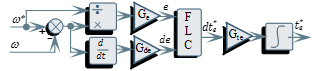
4.3 Fuzzy speed controller
The schematic diagram of the implemented fuzzy speed controller is represented in the Figure 6.
Figure 6. Schematic diagram of the fuzzy speed controller
The inputs of the controller are the error (e) and the change in error (de), the output is the amount of change in the torque reference $\left(d t_{e}^{*}\right)$, an integrator is used to calculate the reference value of the torque.
A new fuzzy rule table (Table 1) was developed and adapted for generator operation, it allows a precise control even at small errors.
Table 1. Proposed fuzzy inference table
|
|
de |
|||||||
|
NB |
NM |
NS |
Z |
PS |
PM |
PB |
||
|
e |
NB |
Z |
PS |
PM |
PB |
PB |
PB |
PB |
|
NM |
NS |
Z |
PS |
PM |
PB |
PB |
PB |
|
|
NS |
NM |
NS |
Z |
PS |
PM |
PM |
PM |
|
|
ZN |
NS |
NS |
NS |
Z |
PS |
PS |
PS |
|
|
ZP |
PS |
PS |
PS |
Z |
NS |
NS |
NS |
|
|
PS |
PM |
PS |
Z |
NS |
NM |
NM |
NM |
|
|
PM |
PS |
Z |
NS |
NM |
NB |
NB |
NB |
|
|
PB |
Z |
NS |
NM |
NB |
NB |
NB |
NB |
|
In this controller, a new method to normalize the error values is implemented, instead of using a constant scaling factor, the normalized value of the error is considered as a percentage, thereby, a big error can be represented as a percentage relative to the reference value. This improves the sensitivity of the controller independently of the reference values range.
The output scaling factor $\left(G_{t e}\right)$ is a very important parameter in the controller, it depends on the system inertia and the machine’s nominal torque.
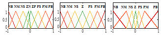
The input and output variables are represented by the fuzzy sets as shown in the Figure 7. In these sets, the letters N P Z S M B refer to Negative, Positive, Zero, Small, Medium and big respectively.
Figure 7. Membership functions
In order to verify the effectiveness of the proposed control scheme, a simulation model has been constructed and simulated under Matlab/Simulink environment. The parameters of the overall system parts are presented in the appendix.
Figure 8. Real and estimated speed of the machine
Figure 9. Speed estimation error evolution
Figure 10. Error between the real and the estimated mechanical angle
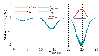
Figure 11. Stator currents: estimated VS real values
In Figure 8, the speed reference, the estimated and the real mechanical speed are shown. The mechanical speed estimation is very accurate with a maximum error of 0.1% from the actual rotor speed as shown in Figure 9, this result can be confirmed by comparison with experimental results reported in [16]. Also, the speed tracking is performant with a maximum error of 0.7% in respect to the speed reference value, these data confirm the efficacy of the proposed fuzzy speed controller and the EKF algorithm. Figure 10 shows the estimation error of the rotor position in mechanical degrees, this error is relatively small and reaches a maximum value of 0.4 % from the actual rotor position, this error induced by estimators is discussed on literature as in paper [25], but effect of the number of pole pairs on control scheme has not been studied. The high number of pole pairs of the machine amplifies the position error causing a large divergence in the estimated $i_{n d}$ current, and an error of 5.5% in the estimation of $i_{n q}$ current relative to the actual value as can be seen in Figure 11. So, even if the precision of the speed estimation is high, errors in position estimation are inevitable, and a high undesirable values of direct axis current can appear.
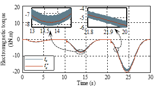
Figure 12. Electromagnetic torque developed by the generator
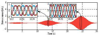
The electromagnetic torque developed by the generator is shown in Figure 12, a good tracking performance can be noted, the error in the position induces a divergence of 5.5 % in high torque values near 25 s, but it can be noted that, making this deviation not dangerous for the system as the machine’s nominal torque is not exceeded. The Figures 13, 14 illustrate the currents in the transformed reference frame, they show that a good tracking behaviour is achieved in term of error and rising time. The currents of the second sub-machine are kept equal to zero, leading to a good current wave quality, as shown in Figure 15, these results are similar to those obtained experimentally [10] with some differences as in the present study the back EMF was supposed perfectly sinusoidal.
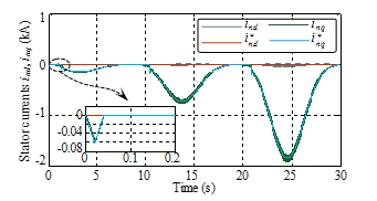
Figure 13. Currents of the first sub-machine
Figure 14. Currents of the second sub-machine
Figure 15. Machine's stator currents
The harmonic content analysis of the phase current shows a variable THD over time depending on the speed of the machine (Figure 16), on low speeds regions (thus, low power), the THD exceeds 5 %, and on high speed regions (thus, high power) the THD becomes very acceptable with values under 5 %, the limit suggested by the IEEE power quality standards. This is caused by the very low inductances of the machine, consequently, the filtering behavior of the windings is bad at low speeds where the impedance of the coils is not sufficiently high (as it depends on the voltage frequency). To enhance the THD, a series connected RL filter can be added between the machine and the converter to help attenuating high frequency harmonics.
Figure 16. Evolution of total harmonic distortion of the machine phase current over time
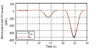
Figure 17. Mechanical power vs DC power
Figure 18. Total effeciency of the considired system
The Figure 17 displays the mechanical power available on the generator’s shaft and the power absorbed by the load, it shows a good efficiency confirmed by Figure 18, the efficiency of the overall system is close to unity, but a small decrease in efficiency is noted when the position error is relatively high, due to apparition of high d axis current.
A tidal stream system has been constructed, modeled and simulated using Matlab/Simulink environment, efforts are made to construct a sensorless system with maximum efficiency and reliability.
The mutual coupling between the machine’s stars have been taken into account, and a proper transformed model is employed to simplify the control of the machine and to minimize the harmonic content of the stator current.
To improve the reliability of the system, sensorless control strategy is adopted using only four AC current sensors and one DC voltage sensor to successfully control the system. The simulation results show a good speed estimation using the EKF estimator, and accurate speed tracking using the proposed fuzzy speed controller. Despite of the high precision of the speed estimation algorithm, the errors in the position estimation are inevitably amplified by the number of poles pairs, causing precision errors of the currents in the transformed reference frame, and a large d axis current can appear, causing a decrease in the system efficiency. The uncontrolled d axis current can cause several damages to the machine, due to overcurrent and saturation, which induces high temperatures, leading to the stator’s insulation failure. A compensation method will be presented in a future work.
We would like to thank the DGRSDT of Algeria for providing necessary subventions to our laboratory.
|
$A_{k}$ |
Discrete machine model matrix |
|
$B_{k}$ |
Discrete input matrix |
|
$C$ |
Dimensionless tides coefficient |
|
$C_{k}$ |
Measurement discrete matrix |
|
$C_{p}$ |
Dimensionless turbine’s power coefficient |
|
$f$ |
Viscose friction coefficient, N.m.s |
|
$G_{d e}$ |
Dimensionless error derivation scaling factor |
|
$G_{e}$ |
Dimensionless error scaling factor |
|
$G_{t e}$ |
Dimensionless torque scaling factor |
|
$i$ |
Current, A |
|
$J$ |
Inertia, kg.m² |
|
$K_{k}$ |
Dimensionless Kalman gain |
|
$L$ |
Inductance, H |
|
$L_{s 0}$ |
Average inductance value, H |
|
$m$ |
Mutual inductance, H |
|
$P$ |
Dimensionless pole pairs |
|
$P_{t}$ |
Turbine power, W |
|
$p$ |
Covariance matrix |
|
$R$ |
Turbine radius, m |
|
$r_{s}$ |
Stator resistance, Ω |
|
$S_{a b c}$ |
Dimensionless converter gates signal |
|
$T(\theta)$ |
Three phase Park’s transformation matrix |
|
$T_{e m}$ |
Electromagnetic torque, N.m |
|
$T_{m}$ |
Turbine torque, N.m |
|
$T_{p}(\theta)$ |
6 phase transformation matrix |
|
$T_{s}$ |
Sampling period, s |
|
$u$ |
Input vector |
|
$v$ |
Voltage, V |
|
$V_{s t} t V_{n t}$ |
Spring and neap tide velocities, m/s |
|
$v_{t}$ |
Tide velocity, m/s |
|
$x$ |
Stat vector |
|
$y_{k}$ |
Output vector |
|
Greek symbols |
|
|
$\varphi$ |
Flux, Wb |
|
$\theta$ |
Electrical position, rad |
|
$\rho$ |
Sea water density, kg/m³ |
|
$\lambda$ |
Dimensionless tip speed ratio |
|
$\omega_{e}$ |
Electrical frequency, rad/s |
|
$\Psi_{P M}$ |
Permanent magnet flux, Wb |
|
$\Omega_{t}$ |
Turbine angular speed, rad/s |
|
$\Omega$ |
Machine’s angular speed, rad/s |
|
Subscripts |
|
|
$n d$ |
First submachine d axis component |
|
$n q$ |
First submachine q axis component |
|
$a d$ |
Second submachine d axis component |
|
$a q$ |
Second submachine q axis component |
|
$k, k-1$ |
Actual and previous step |
|
Superscripts |
|
|
$\wedge$ |
Estimated variable |
Table 2. Turbine parameters
|
R |
8 m |
|
Rated marine current speed |
2.5 m/s |
Table 3. Generator and gearbox parameters
|
Generator rated power |
700 kW |
|
$r_{s}$ |
66.040 mΩ |
|
$m$ |
22.84 µH |
|
$L_{s 0}$ |
53,758 µH |
|
$\Psi_{P M}$ |
0.3244 Wb |
|
$P$ |
11 |
|
$f$ |
0 N/m |
|
Gearbox ratio |
21.1 |
Table 4. Control system parameters
|
EKF Q covariance matrix |
diag([0.03 0.03 0.03 0.03 0.005]) |
|
EKF R covariance matrix |
1e5*diag([1 1 1 1]) |
|
$i_{n q}$ PI regulator |
Kp = 1.89, Ki = 8.51 |
|
$i_{n d}$ PI regulator |
Kp = 25.14, Ki = 13.87 |
|
$i_{a d}$ and $i_{a q}$ PI regulator |
Kp = 3.89, Ki = 2.34 |
[1] Meisen, P., Hammons, T. (2005). Harnessing the untapped energy potential of the oceans: Tidal, wave, currents and OTEC. In IEEE Power Engineering Society General Meeting, 1853-1854. https://doi.org/10.1109/PES.2005.1489449
[2] Hammons, T.J. (1993). Tidal power. Proc IEEE, 81(3): 419-433. https://doi.org/10.1109/5.241486
[3] Benbouzid, M., Astolfi, J.A., Bacha, S., Charpentier, J. F., Machmoun, M., Maître, T., Roye, D. (2011). Concepts, modélisation et commandes des hydroliennes. Institut de Recherche de l’École navale (IRENAV), http://hdl.handle.net/10985/8832
[4] Levi, E., Bojoi, R., Profumo, F., Toliyat, H.A., Williamson, S. (2007). Multiphase induction motor drives–a technology status review. IET Electric Power Applications, 1(4): 489-516. https://doi.org/10.1049/iet-epa:20060342
[5] Mayouf, M., Bakhti, H. (2019). Monitoring and control of a permanent magnet synchronous generator-based wind turbine applied to battery charging. Energy Sources, Part A: Recovery, Utilization, and Environmental Effects, 1-16. https://doi.org/10.1080/15567036.2019.1666934
[6] Hannan, M.A., Ali, J.A., Mohamed, A., Hussain, A. (2018). Optimization techniques to enhance the performance of induction motor drives: A review. Renewable and Sustainable Energy Reviews, 81: 1611-1626. https://doi.org/10.1016/j.rser.2017.05.240
[7] Karttunen, J., Kallio, S., Peltoniemi, P., Silventoinen, P., Pyrhönen, O. (2012). Dual three-phase permanent magnet synchronous machine supplied by two independent voltage source inverters. In International Symposium on Power Electronics Power Electronics, Electrical Drives, Automation and Motion, 741-747. https://doi.org/10.1109/SPEEDAM.2012.6264448
[8] Mahmoudi, L.N.M.O. (2010). Vector control with optimal torque of a salient–pole double star synchronous machine supplied by three–level inverters. Journal of Electrical Engineering, 61(5): 257-263. https://doi.org/10.2478/v10187-010-0037-0
[9] Kallio, S., Andriollo, M., Tortella, A., Karttunen, J. (2012). Decoupled dq model of double-star interior-permanent-magnet synchronous machines. IEEE Transactions on Industrial Electronics, 60(6): 2486-2494. https://doi.org/10.1109/TIE.2012.2216241
[10] Karttunen, J., Kallio, S., Peltoniemi, P., Silventoinen, P., Pyrhönen, O. (2013). Decoupled vector control scheme for dual three-phase permanent magnet synchronous machines. IEEE Transactions on Industrial Electronics, 61(5): 2185-2196. https://doi.org/10.1109/TIE.2013.2270219
[11] Knudsen, H. (1995). Extended Park's transformation for 2/spl times/3-phase synchronous machine and converter phasor model with representation of AC harmonics. IEEE Transactions on Energy Conversion, 10(1): 126-132. https://doi.org/10.1109/60.372577
[12] Nak, H., Gülbahce, M.O., Gokasan, M., Ergene, A.F. (2015). Performance investigation of extended Kalman filter based observer for PMSM using in washing machine applications. In 2015 9th International Conference on Electrical and Electronics Engineering (ELECO), pp. 618-623. https://doi.org/10.1109/ELECO.2015.7394564
[13] Malinowski, M. (2001). Sensorless control strategies for three-phase PWM rectifiers. Poland, Warsaw University of Technology.
[14] Blaabjerg, F., Pedersen, J.K., Jaeger, U., Thoegersen, P. (1997). Single current sensor technique in the DC link of three-phase PWM-VS inverters: A review and a novel solution. IEEE Transactions on Industry Applications, 33(5): 1241-1253. https://doi.org/10.1109/28.633802
[15] Agrawal, J., Bodkhe, S. (2019). Speed sensorless vector controlled SMPMSM drive based on modified MRAS with single current sensor. IETE Journal of Research, 1-15. https://doi.org/10.1080/03772063.2019.1627915
[16] Park, J.B., Wang, X. (2018). Sensorless direct torque control of surface-mounted permanent magnet synchronous motors with nonlinear Kalman filtering. Energies, 11(4): 969. https://doi.org/10.3390/en11040969
[17] Wicaksono, N.A., Harini, B.W., Yusivar, F. (2018). Sensorless PMSM control using fifth order EKF in electric vehicle application. In 2018 5th International Conference on Electrical Engineering, Computer Science and Informatics (EECSI), pp. 254-259. https://doi.org/10.1109/EECSI.2018.8752759
[18] Sahraoui, K., Ameur, A., Kouzi, K. (2018). Performance enhancement of sensorless speed control of DSIM using MRAS and EKF optimized by genetic algorithm. In 2018 International Conference on Applied Smart Systems (ICASS), 1-8. https://doi.org/10.1109/ICASS.2018.8651996
[19] Elghali, S.E.B., Balme, R., Le Saux, K., Benbouzid, M.E.H., Charpentier, J.F., Hauville, F. (2007). A simulation model for the evaluation of the electrical power potential harnessed by a marine current turbine. IEEE Journal of Oceanic Engineering, 32(4): 786-797. https://doi.org/10.1109/JOE.2007.906381
[20] Benbouhenni, H., Boudjema, Z., Belaidi, A. (2020). Power control of DFIG in WECS using DPC and NDPC-NPWM methods power control of DFIG in WECS Using DPC and NDPC-NPWM methods. Math Model Eng Probl, 7: 223-236. https://doi.org/10.18280/mmep.070208
[21] Hau, E. (2013). Wind turbines: Fundamentals, technologies, application, economics. Springer Science & Business Media. https://doi.org/10.1007/978-3-642-27151-9.
[22] Zhou, Z., Scuiller, F., Charpentier, J.F., Benbouzid, M.E.H., Tang, T. (2014). Power control of a nonpitchable PMSG-based marine current turbine at overrated current speed with flux-weakening strategy. IEEE Journal of Oceanic Engineering, 40(3): 536-545. https://doi.org/10.1109/JOE.2014.2356936
[23] Levi, E. (2008). Multiphase electric machines for variable-speed applications. IEEE Transactions on Industrial Electronics, 55(5): 1893-1909. https://doi.org/10.1109/TIE.2008.918488
[24] Amirouche, E., Lyes, K., Kaci, G., Djamal, A. (2019). Simulation study of the dual star permanent magnet synchronous machine using different modeling approaches. In International Conference on Electrical Engineering and Control Applications, pp. 389-405. https://doi.org/10.1007/978-981-15-6403-1_27
[25] Khlaief, A., Boussak, M., Gossa, M. (2013). Model reference adaptive system based adaptive speed estimation for sensorless vector control with initial rotor position estimation for interior permanent magnet synchronous motor drive. Electric Power Components and Systems, 41(1): 47-74. https://doi.org/10.1080/15325008.2012.732657